Critical literature review
Here we are commenting on some published papers in the literature, trying to trace back the fate of the equations.
On this page
Manabe and Wetherald (1967) convective adjustment
Houghton (1977) Radiative equilibrium
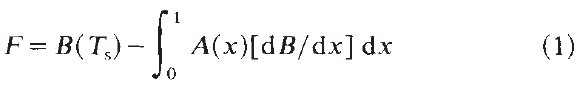
Raval and Ramanathan (1989) Observational determination of the greenhouse effect
Stephens and Greenwald (1991) Radiation budget and atmospheric hydrology
Ramaswamy et al. (2019) Radiative forcing
GFDL Atmospheric Model 4 (2019)
Ramaswamy (2023 Sun-Climate Symposium)
Manabe and Wetherald (1967)
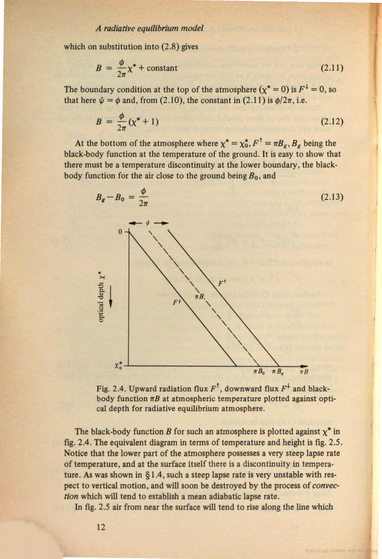
Emden (1913) realized that, applied for the Earth's atmosphere, Eq. (11) requires a discontinuity ('Temperatursprung') between the temperature of the surface and the lowest atmospheric layer (about 20°C), but in the same sentence he notes that this jump in temperature is greatly diminished by heat conduction and evaporation. This way, Emden discovered radiative-convective equilibrium: convective fluxes are not free parameters in the global energy balance but stricktly constrained to the size of discontinuity, that is, to the net radiation surplus at the surface: Sensible heat (convection-conduction) + Latent heat (evaporation) = A – E = ΔA.
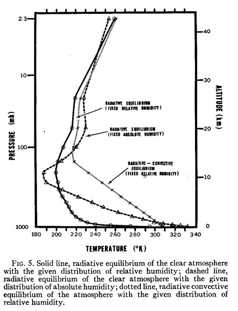
Manabe and Strickler (1964, Fig. 4.) and Manabe and Wetherald (1967, Fig. 5.) compute correctly the magnitude of this discontinuity,

Sensible heat (convection+conduction) + Latent heat (evaporation) = A – E = ΔA = A0/2 .
Manabe does not mention this constraint on convection in any of his writings. We recall that the euality is verified on global mean clear-sky data of CERES EBAF Ed2.8 by a difference of 0.6 Wm-2, on EBAF Ed41 by 2.3 Wm-2, on EBAF Ed4.2 by 2.4 Wm-2; the all-sky version is valid by a difference of 0.1 Wm-2 on the GEWEX energy budget (Stephens et al., BAMS, 2023).
[Historical speculation: It is possible that Manabe and Strickler (1964) were aware of Emden's work as it appeared by translation in the Monthly Weather Review (1916), but were not of Schwarzschild's original paper. Emden finds the discontinuity (temperature jump) in radiative equilibrium, but in his paper there is no mention of the other side of the equality (A0/2), which is evident for the first sight in Schwarzschild (1906). Had Manabe and Strickler seen the Schwarzschild paper, they would have certainly found the full relationship, and they constrain their convective adjustment not only to ΔA but to A0/2 as well.]
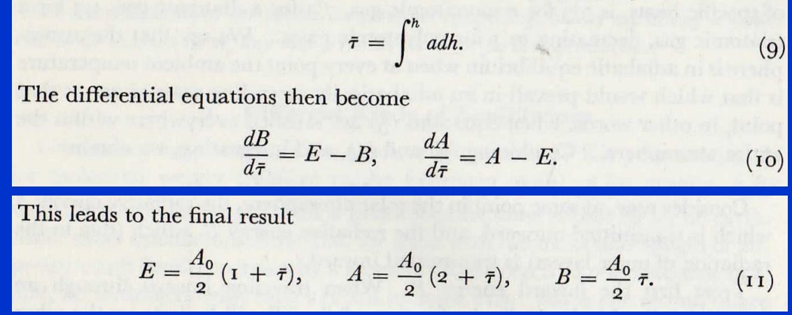
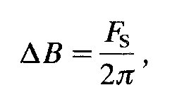
Houghton (1977) in his book The Physics of Atmospheres gives a radiative equilibrium model and a direct derivation of the "net" relationship:
 .
.Contrary to this clear determination, this constraint is not taken into account later in the book when the enhanced greenhouse effect, water vapor feedback and climate sensitivity is discussed.
Foreword:
- "concerns have prompted a number of investigations of the implications of increasing carbon dioxide. Their consensus has been that increasing carbon dioxide will lead to a warmer earth."
- "If carbon dioxide continues to increase, the study group finds no reason to doubt that climate changes will result"
Preface:
- "Our charge was to identify the principal premises on which our current understanding of the question is based"
Contents:
1 Summary and Conclusions:
- "We have examined the principal attempts to simulate the effects of increased atmospheric C02 on climate".
-" To summarize, we have tried but have been unable to find any overlooked or underastimetad physical effects"
2 Carbon in the atmosphere
3 PHYSICAL PROCESSES IMPORTANT FOR CLIMATE AND CLIMATE MODELING
3.1 Radiative Heating
3.2 Cloud Effects
3.3 Oceans
4 MODELS AND THEIR VALIDITY
4.1 Three-Dimensional General Circulation Models.
Physical processes: Radiative heating.
3.1.1 Direct radiative effects
This is the point where the connection between CO2 concentration and radiation should be established.
"An increase of the C02 concentration in the atmosphere increases its absorption and emission of infrared radiation and also increases slightly its absorption of solar radiation. For a doubling of atmospheric C02 , the resulting change in net heating of the troposphere, oceans, and land (which is equivalent to a change in the net radiative flux at the tropopause) would amount to a global average of about ΔQ = 4 Wm-2 if all other properties of the atmosphere remained unchanged. This quantity, ΔQ, has been obtained by several investigators, for example, by Ramanathan et al. ( 1979),"
Let's see, Ramanathan et al. (1979):
"A number of published model studies have examined the climati effects of increased tmospheric CO2 concentrations. These studies have employed a hierarchy of climate models, including the one-dimensional radiative-convective model (Manabe and Wetherald 1967) ... and three-dimensionsal general circulation model (Manabe and Wetherald 1975). ... All of these model studies show that increased CO2 would produce an increase in surface and tropospheric temperatures.
a Radiative transfer model
The model used for this study is described in detail by Ramanathan and Dickinson (1979). This model is based on that developed by Ramanathan (1976)... "
Ramanathan (1976), A simplified Radiative-Convective Model:
"Detailed radiative transfer analysis for the earth's atmosphere have been presented by Ellingson (1972", An infrared radiative transfer model, PhD thesis)...
Ellingson (1978), Description of the model: Plane-parallel, LTE, LW in at TOA = 0, no scatter.
Net flux:
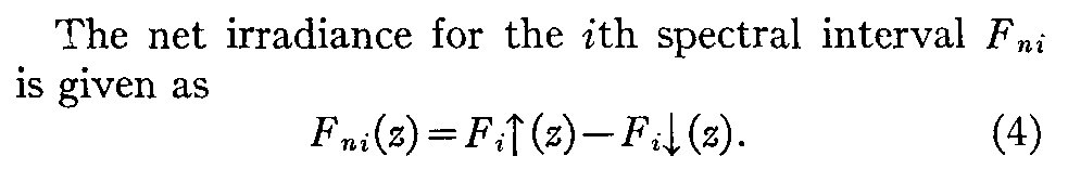
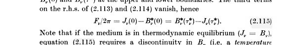
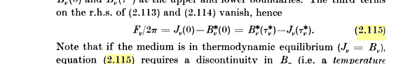
For a review of the early works refers to Goody (1964, Atmospheric radiation: Theoretical basis). This book derives the Eddington plane-parallel approximation of Schwarzschild's integral equation and finds (Eq. 2.115):
This way, the circle is closed: at the root of the references there is the constraint being missed (overlooked) by the Charney report and all of the subsequent studies, including each of the IPCC reports (1990-2022).
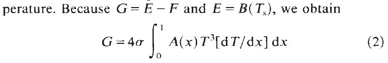
Raval and Ramanathan (1989) Observational determination of the greenhouse effect (Nature 42: 758-761). G is correctly defined as G = SFC LW emission – TOA LW emission,
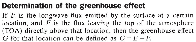
OLR is not Surface emission – Atmospheric absorption (which gives surface transmitted irradiance, window radiation).
Therefore Eq. (2) also erroneous, describing atmospheric absorption:
G = Surface emission – TOA emission = (Surface emission – WIN) – (TOA emission – WIN) = Atmospheric LW absorption – Atmospheric LW upward emission.
This error is repeated in Ramanathan and Inamdar (2006):
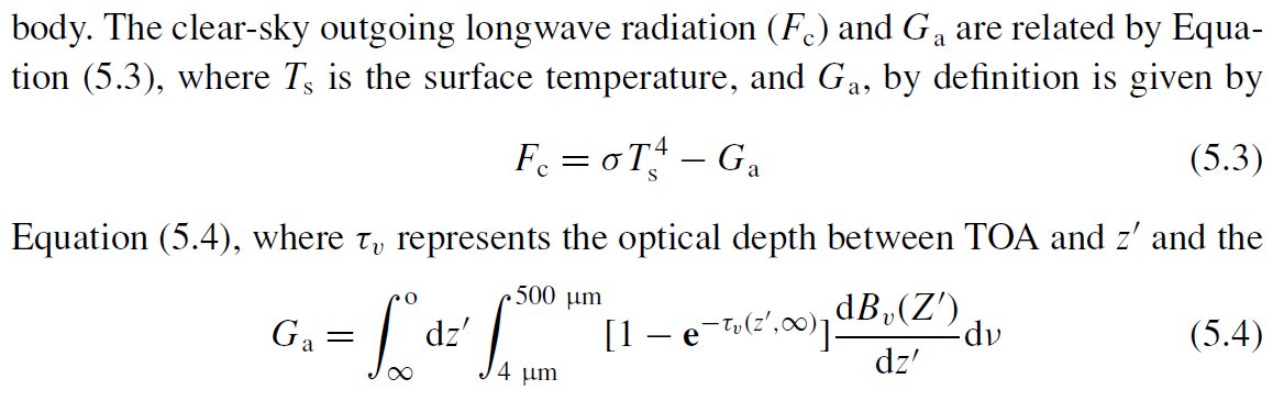
Stephens and Greenwald (1991) The Earth's radiation budget and its relation to atmospheric hydrology. Observations of the clear-sky greenhouse effect.
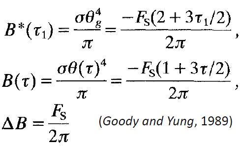
To establish the relation between Earth's radiation budget and the hydrological activity, the paper uses Schwarzschild's plane-parallel equations, taken from Michalas (1978) and Goody and Yung (1989):
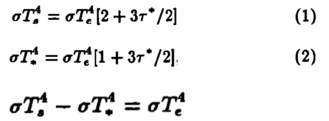
But as it can be seen, a division by two is missing from the right-hand side in each equations; correctly:
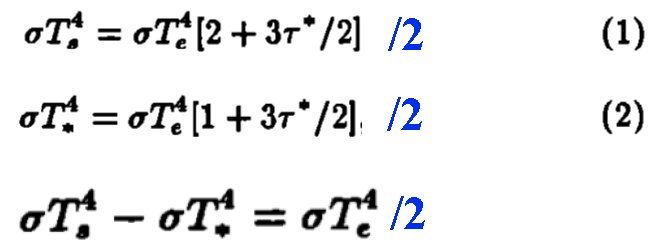
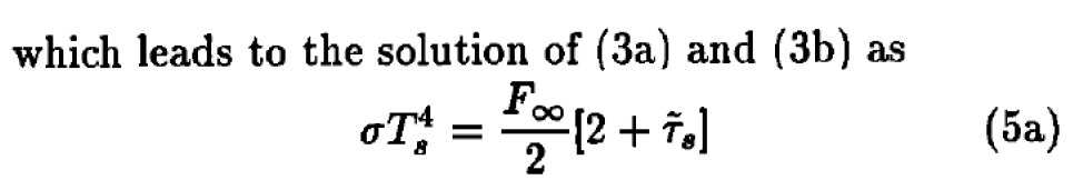
but in that paper the equation for the net radiation at the surface was not formed. This was the point in the literature where a researcher came the closest to realize the constraint. By missing it, all the subsequent studies and assessment reports proceeded with an unconstrained hydrological cycle, unlimited climate sensitivity and greenhouse enhancement.
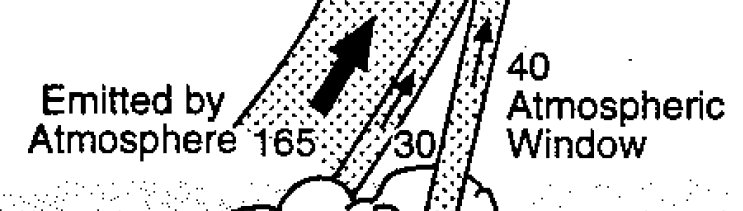
Kiehl and Trenberth (1997). I was always wondering what that '30' really represents in the diagarm of KT97.
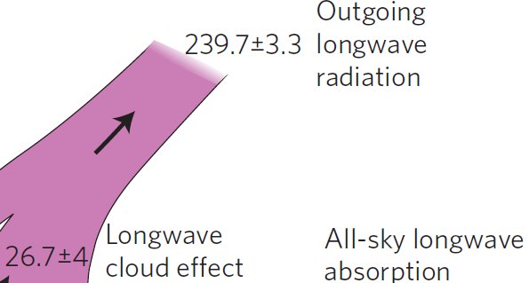
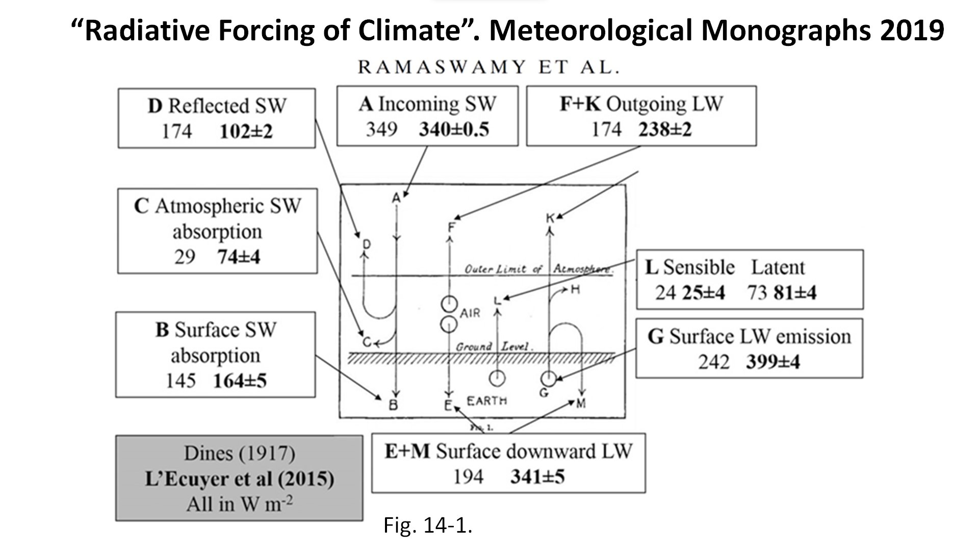
Ramaswamy et al. in AMS Meteorological Monograph (2019, Chapter 14, Radiative forcing of climate), say: "Arrhenius (1896) made the quantitative connection to estimate the surface temperature increase due to increases in CO2. ... Arrhenius’ systematic investigation and inferences have proven to be pivotal in shaping the modern-day thinking and computational modeling of the climate effects due to CO2 radiative forcing." ... "What we term as RF of climate change today can be regarded as a result of this early thinking about the surface–atmosphere heat balance." An early estimate of Earth's global average energy budget of Dines (1917) is given (Figure 14-1), providing a comparison to one modern analysis (L'Ecuyer et al. 2015):
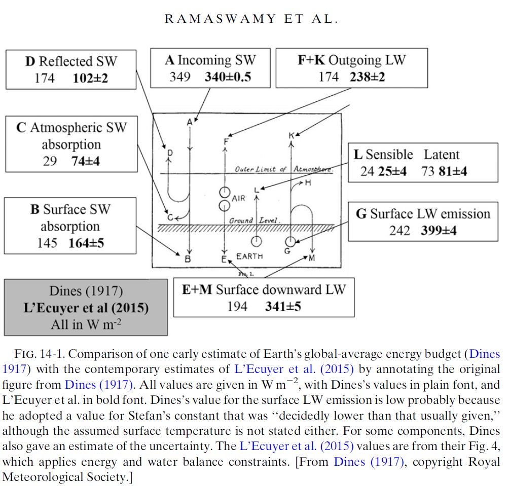
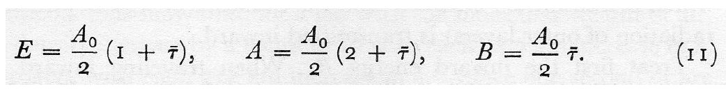
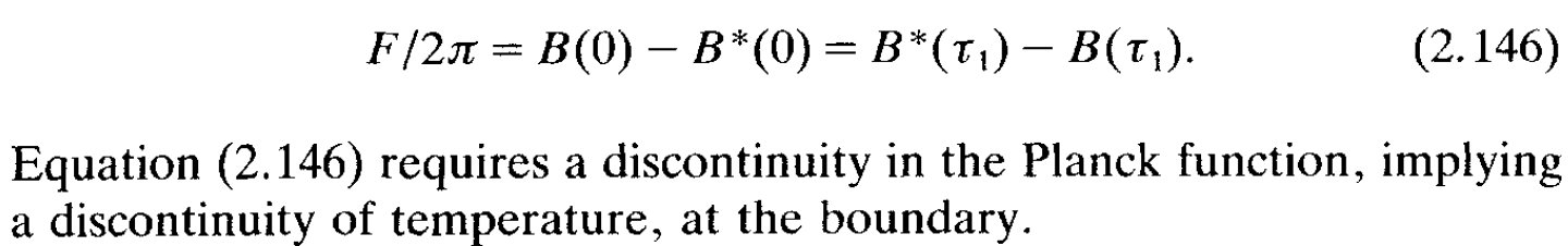
But another line of theoretical thinking was radiative equilibrium and radiation transfer, from Schuster (1905), Schwarzschild (1906) and others. Note that in the 20-page long reference list of Ramaswamy et al. (2019), containing about one thousand entries, Schwarzschild's name does not occur. Instead, on the same page (14.3), Rawaswamy et al. (2019) refer to chapter 2 in Goody and Yung (1995, Atmospheric radiation, Theoretical basis) for the formalism of atmospheric longwave radiative transfer, where Goody and Yung refer back to Schwarzschild's equation as the theoretical fundament of their whole work. But Ramaswamy et al. (2019) do not recognize that equation (2.146) in chapter 2 of Goody and Yung,
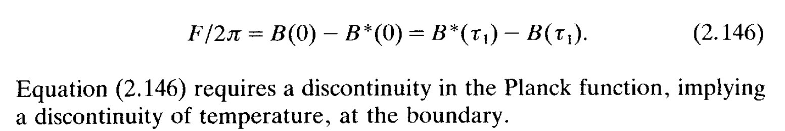
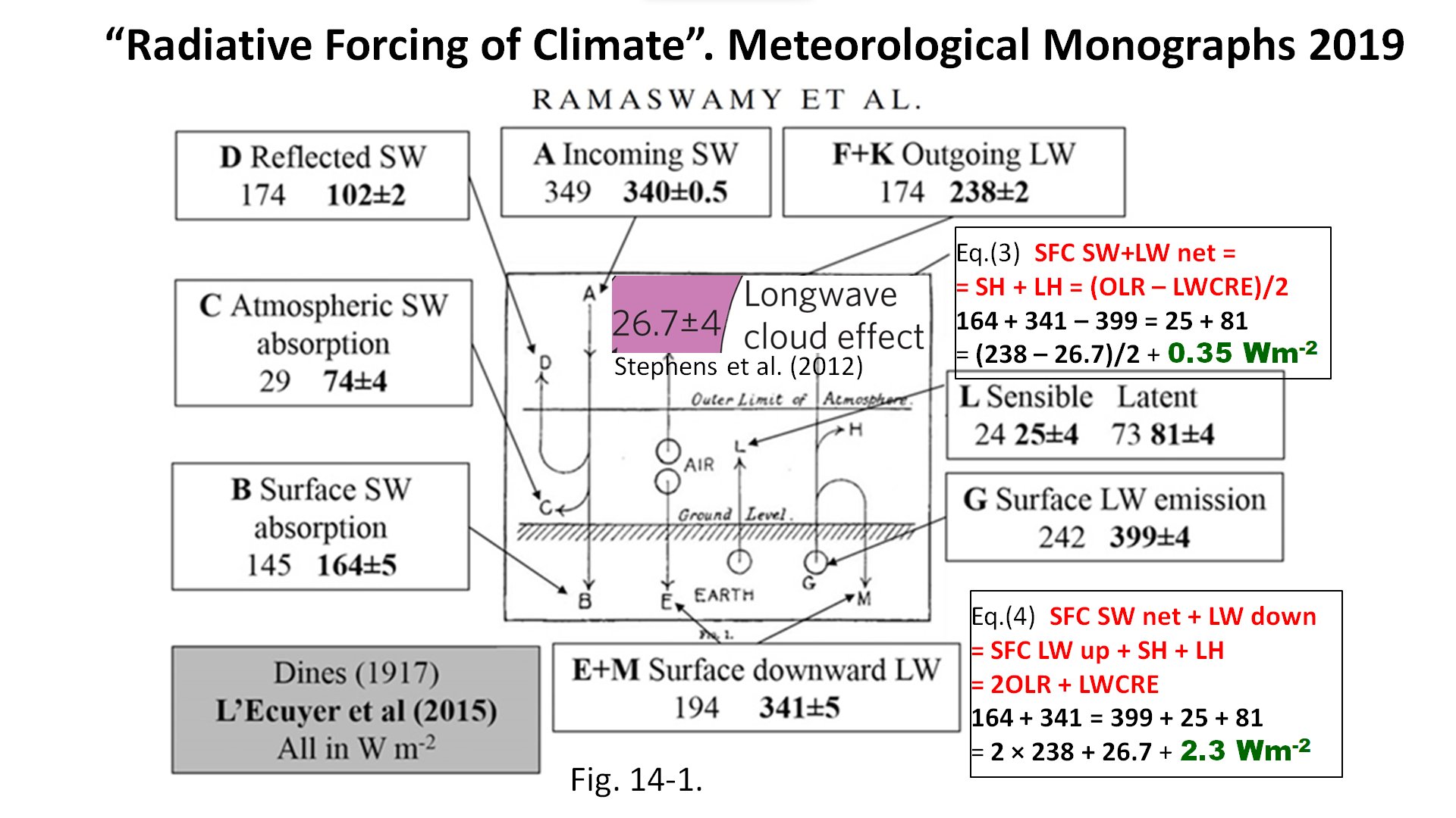
describes the net constraint equation for clear-sky conditions, connecting the discontinuity at the surface, and the corresponding net radiation unequivocally to half of OLR in the clear-sky, while the all-sky version of this equation is satisfied by their reference study L'Ecuyer et al. (2015) by a difference of 0.35 Wm-2. The total version of the equation is valid by a difference of 2.30 Wm-2 [LWCRE is taken from a contemporary study by the same authors (Graeme Stephens, Tristan L'Ecuyer and others) as 26.7 Wm-2]:
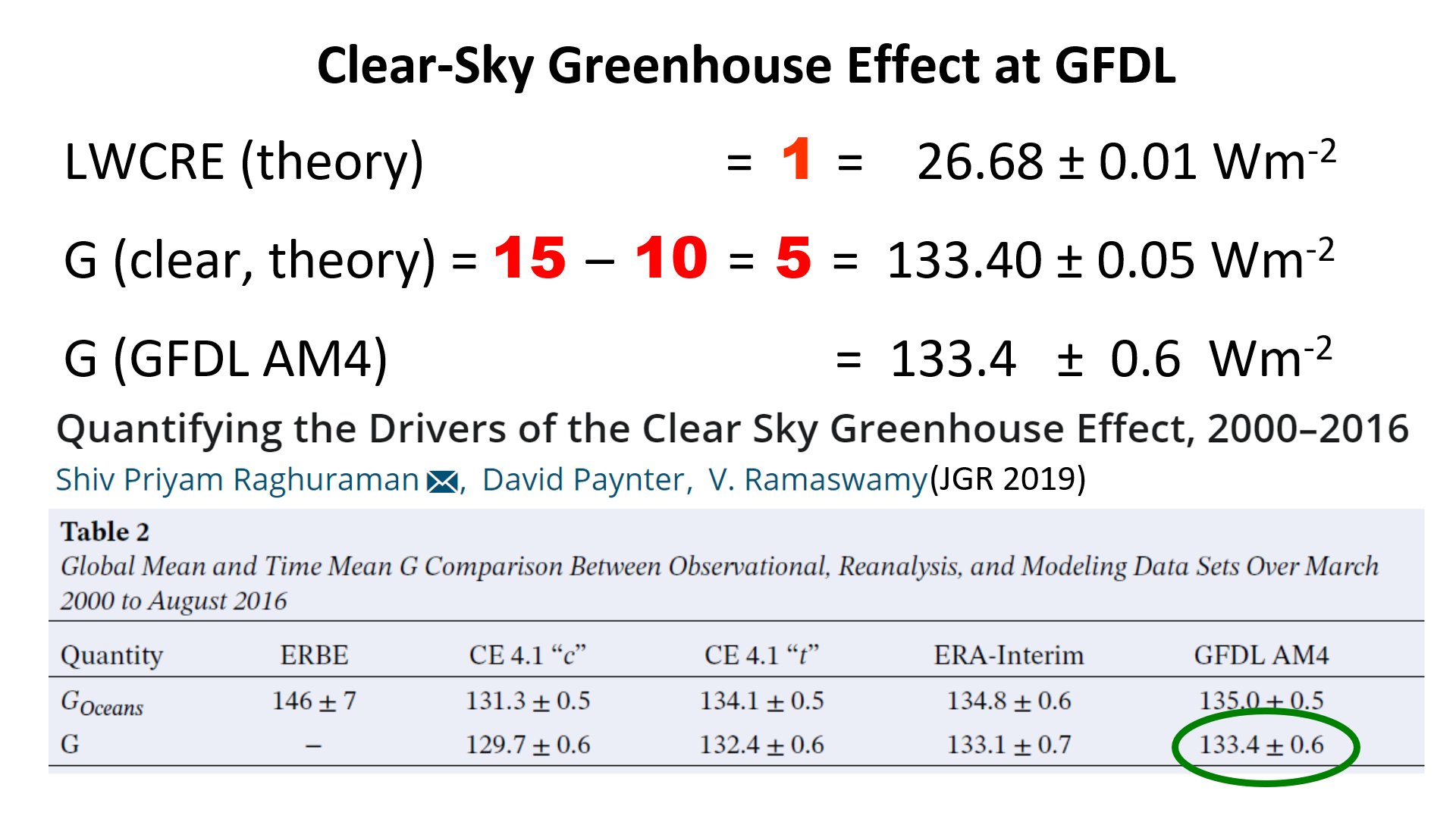
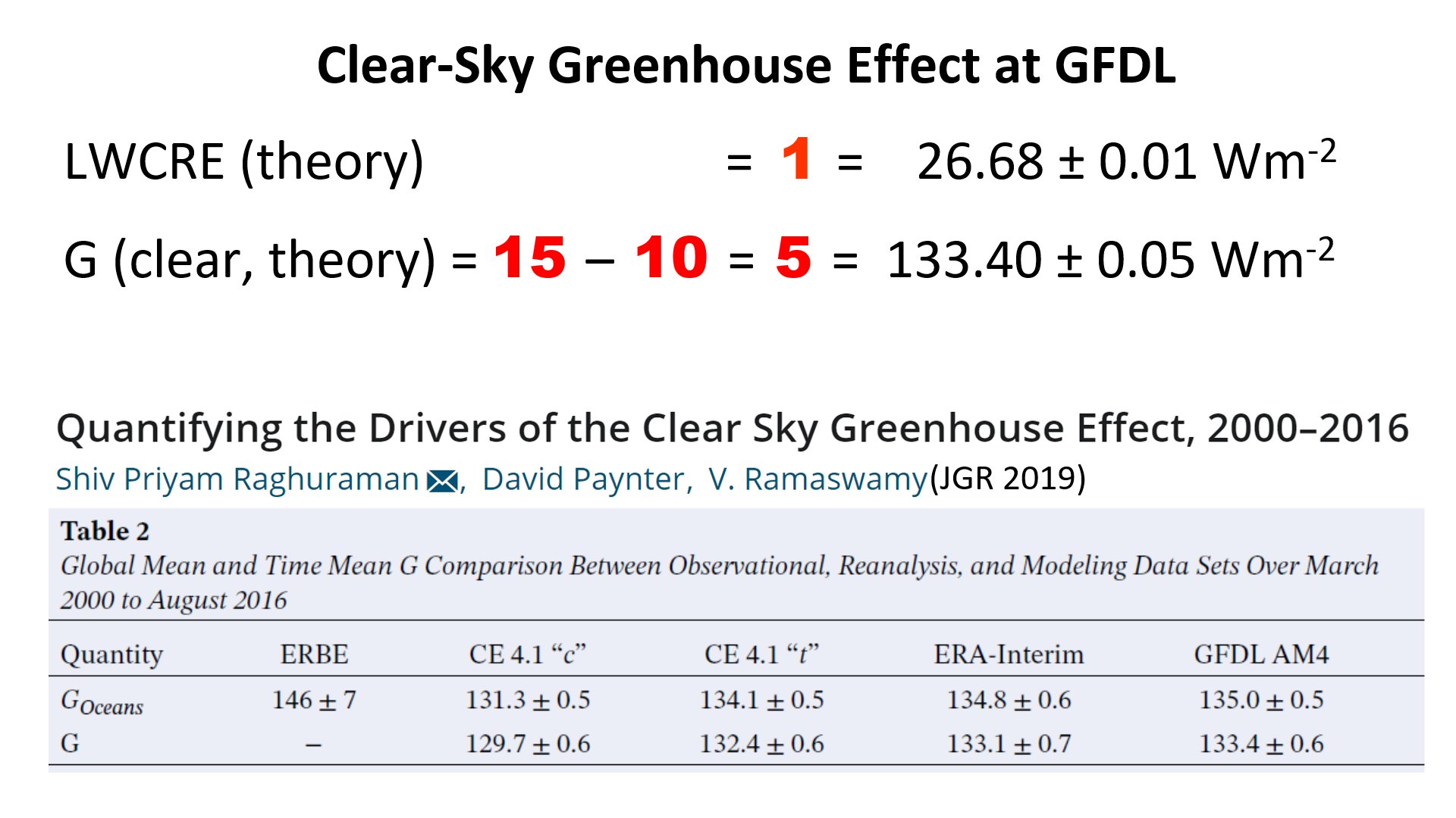
Raghuraman, Paynter and Ramaswamy (2019), quantifying the antropogenic drivers and feedbacks of the clear-sky greenhouse effect and its sensitivity to the different factors, refer to their accepted G value from the GFDL Atmospheric Model 4, as G = 133.4 ± 0.6 Wm-2. Let us point out that this value is exactly equal to our geometric greenhouse effect, derived without any reference to the gaseous composition of the atmosphere or the temperature lapse rate. Using the best fit of the unit flux on the CERES dataset as ONE UNIT = 26.68 ± 0.01 Wm-2, we have:
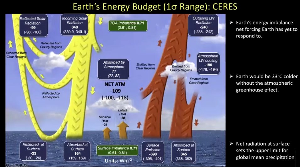
Dr. Norman Loeb, in a recent presentation at JPL Center for Climate Sciences (Virtual Mini-Symposium on Climate and Radiation Monitoring, April 18, 2022) showed an updated CERES energy budget diagram:
Hansen et al. (2005), when coining the term 'Earth's Energy Imbalance', estimate GHG and aerosol forcing at TOA as 0.85 ± 0.15 Wm-2, while refer to the observed ocean heat gain as 0.86 ± 0.12 Wm-2; the transfer function is not taken into account. Meyssignac et al. (2019) and Stephens et al. (2023) note that "none of the techniques available today enable us to estimate the EEI with the perceived required accuracy less than ±0.3 W m−2, let alone with an aspirational accuracy of ±0.1 W m−2."
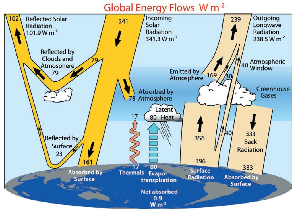
Fasullo and Trenberth (2008) define the net downward radiation (RT) at TOA, and when partition it into its components, they should have declared that it causes (5/3)RT imbalance at the surface. Trenberth, Fasullo and Kiehl (2009), when incorporating the imbalance concept into their global energy flows, still miss the concept: their Incoming solar radiation is 341.3 Wm-2, Reflected solar radiation is 101.9 Wm-2, that is, their Absorbed solar radiation is 239.4 Wm-2, while outgoing LW is 238.5 Wm-2, indicating an imbalance at TOA = 0.9 Wm-2, same as the surface Net absorbed; f(all) is not utilized.
IPCC AR5 was even less careful, they give 0.6 Wm-2 residual at the lower boundary, but indicating 1 Wm-2 imbalance at the upper boundary, thus having exactly the opposite ratio (TOA/SFC = 5/3) as would be justified. While we understand the existence of huge uncertainties in these estimates from very different data sources, the median ought to be as accurate as possible, and energy conswervation should be strictly satisfied.
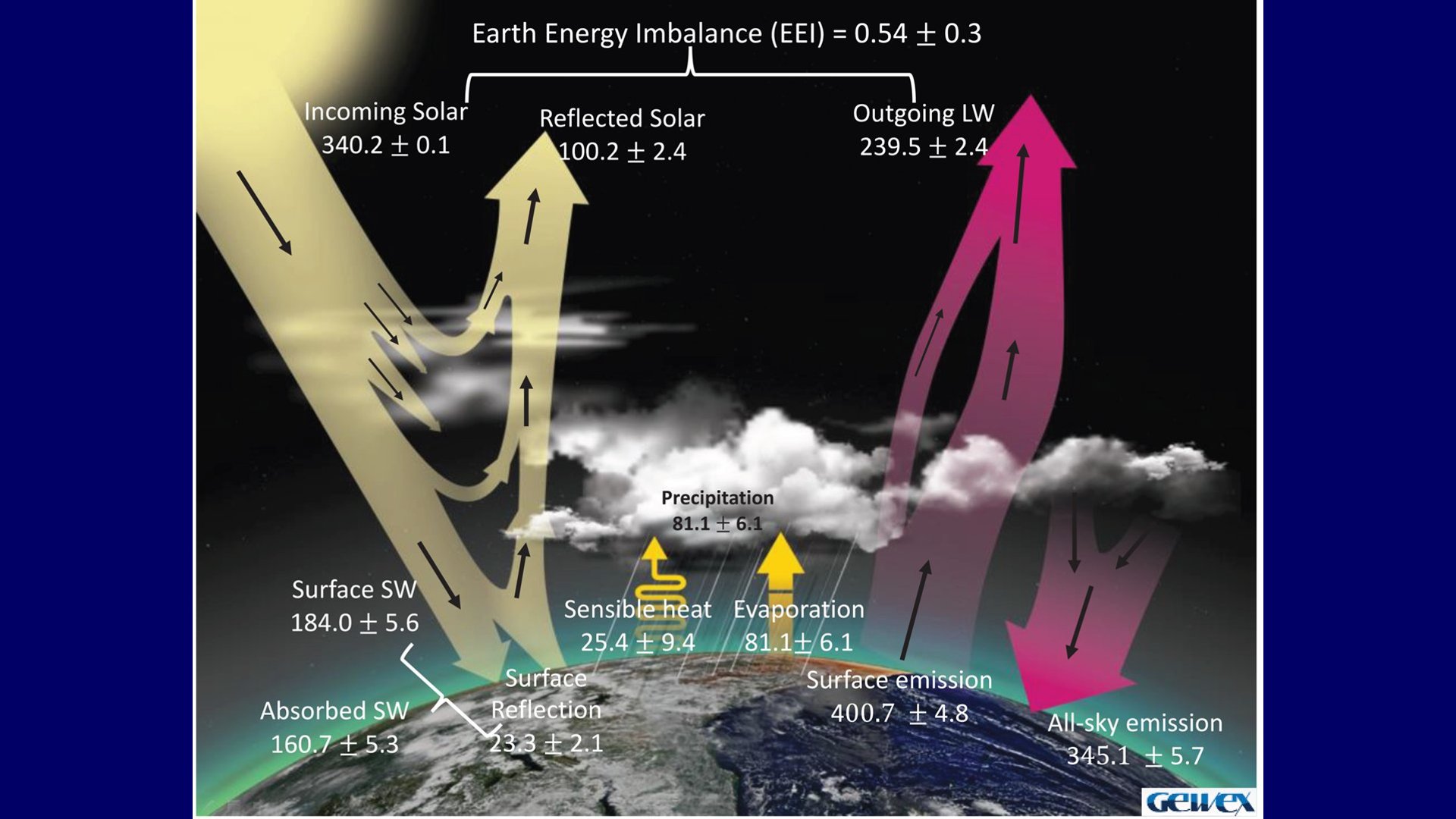
The GEWEX diagram in BAMS (Stephens et al. 2023) has 0.54 Wm-2 EEI at TOA, adjusted to their accepted 0,9 Wm-2 ocean heat content increase, since 0.9 = (5/3) × 0.54.
For the clear-sky case, the transfer factor is 2.
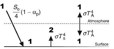
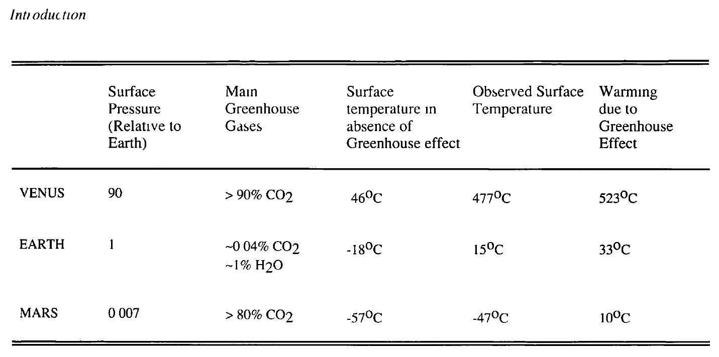
About the second point, Dr. Loeb said :"Within the atmosphere, we know that greenhouse gases are pretty critical, the Earth would be 33 degrees colder without the greenhouse gases". Let us recall here again that the simplest greenhouse geometric arrengement, the single-layer atmospheric model, see Hartmann 2016, Fig. 2.3 below (or visit again our assessment of Trenberth's greenhouse model, which is the same geometry), reproduces this value without any reference to the amount of the greenhosue gases in the atmosphere:
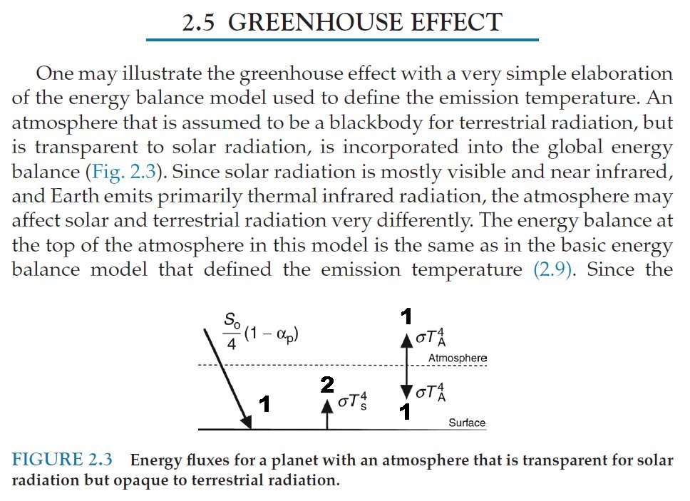
Introducing our Eq. (1) from Schwarzschild (1906, Eq. 11) or Goody (1964, Eq. 2.115) or Houghton (1977, Eq. 2.13) or Goody and Yung (1989, Eq. 2.146, see above):
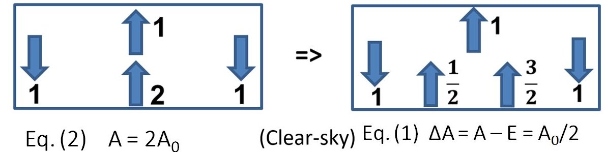
and extending the system to the all-sky by introducing L as LWCRE:
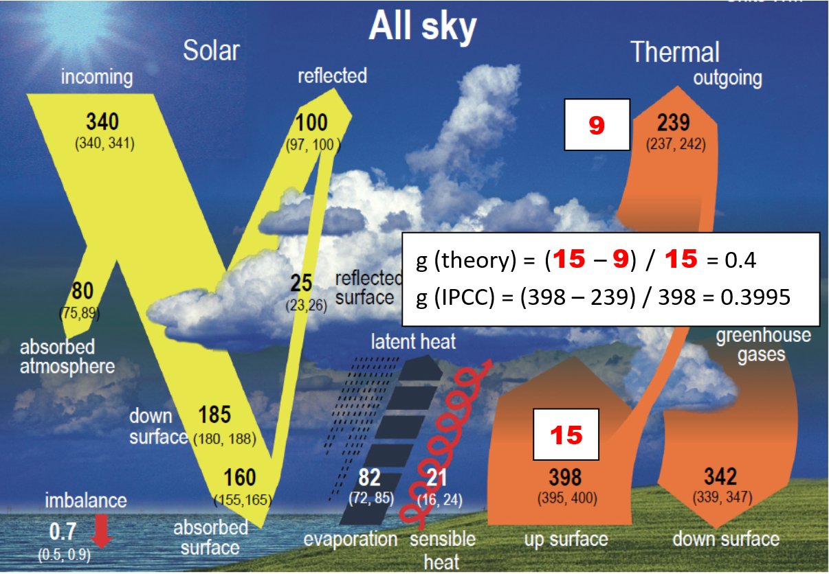
we will have a geometric arrangement, where the greenhouse effect is generated by the simplest radiative principles involved in Hartmann's or Trenberh's figure above. The all-sky greenhouse effect is 15 – 9 = 6 units, with 1 unit = 26.68 Wm-2 as the best fit on the CERES 22-year data, leading to 15 units = 400.20 Wm-2 = 289.85°C at the surface, 9 units = 240.12 Wm-2 = 255.10 °C as effective emission temperature, and a theoretical greenhouse effect of 34.75°C. The estimate of surface emission as 398 Wm-2 and outgoing LW = 240 Wm-2 leads to 289.45 °C – 255.07 °C = 34.38 °C as greenhouse temperature.
[Actually, we were unable to identify any reliable energy budget estimate which would result in a 33 degree greenhouse temperature, mentioned by NASA, World Meteo Organization and elsewhere. CERES EBAF Edition 4.2, 22 years of data (April 2000 - March 2022) has ULW = 398.42 Wm-2 and OLR = 240.33 Wm-2, so G = 158.09 Wm-2, equivalent to 34.37 °C. Even the original Kiehl and Trenberth 1997 diagram, served as FAQ 1.1, Figure 1 for the IPCC AR4 Report in 2007, with its data of 390 Wm-2 and 235 Wm-2 results in 34.26 °C. Each is less than the theoretical, but each is higher than 34 °C.]
Greenhouse gases and the lapse rate do not play a decisive role, their task is to maintain the "plate state". With enough free ocean surfaces, for any amount of non-condensing GHGs, water vapour will be able to do the rest of job.
About the third point, "Net radiation at the surface sets the upper limit for global mean precipitation"; yes, but here we refer back to the theoretical constraints on the convective fluxes: net radiation sets even more: it constrains the total convective activity (including the hydrological cycle) to half of OLR in the clear-sky and to (OLR – LWCRE)/2 in the all-sky, validated with a 0.09 Wm-2 difference on the published GEWEX diagram (see our GEWEX BAMS chapter).
For the sake of the Reader, we reproduce here Dr. Loeb's diagram projected with the integer system:
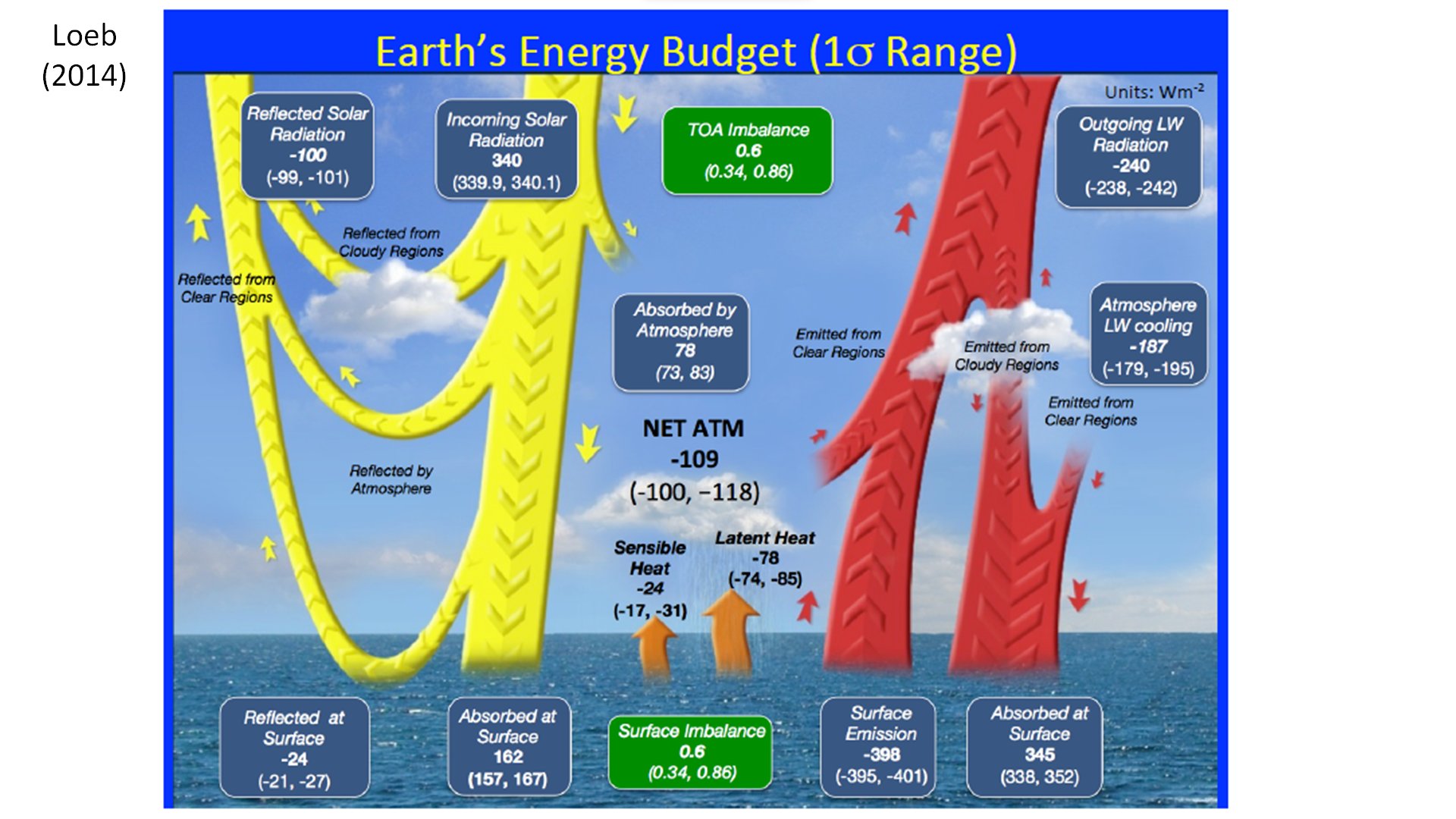
Each flux component fits to its integer position within the stated range of uncertainty.
TOA fluxes: zero difference. The largest deviation is 2.67 Wm-2 (Reflected at Surface).
By their data, the greenhouse temperature is 34.38 °C, compared to the theoretical (purely geometric) 34.75 °C,
and the difference of NET ATM (109 Wm-2) from the theoretical constraint (OLR – LWCRE)/2 = 107.1 Wm-2 is 1.9 Wm-2.
Jeevanjee, Held and Ramaswamy reviewed the work of "Syukoro" (sic, correctly: Syukuro) Manabe on Radiative–Convective Equilibrium (BAMS 2022) and identified its first crucial ingredient as "a tight convective coupling of the surface to the troposphere"... "the resultant coupling of surface and TOA energy balance is the essence of ingredient 1". They continue: "in pure radiative equilibrium the atmosphere in the global mean is gravitationally unstable in a layer adjacent to the surface. Atmospheric motions transport heat upward to balance the radiative destabilization." They hail Manabe's work to realize that "changes in the surface energy balance are dominated by changes in convective fluxes that are constrained to take on values consistent with a small air–surface temperature jump" (emphasis in the original).
But the paper does not mention that this constraint on the convective fluxes (to be equal to the "radiative destabilization" in pure radiative equilibrium) is only one half of the constraintment: the equation that prescribes the temperature jump constrains its magnitude to half of the TOA LW flux (in clear-sky): ΔA = A0/2. As mentioned above, Manabe and Strickler (1964) and Manabe and Wetherald (1967) calculate correctly the size of this temperature jump (of about 20 °C), but do not recognize taht it is unequivocally constrained to half of OLR. The review paper of Jeevanjee et al. misses this lack of recognition as well.
The First Assessment Report (1990) declares at the very beginning:
" EXECUTIVE SUMMARY
We are certain of the following:
• there is a natural greenhouse effect which already keeps the Earth wanner than it would otherwise be
• emissions resulting from human activities are substantially increasing the atmospheric concentrations of the greenhouse gases carbon dioxide, methane, chlorofluorocarbons (CFCs) and nitrous oxide. These increases will enhance the greenhouse effect, resulting on average in an additional warming of the Earth's surface The main greenhouse gas, water vapour, will increase in response to global warming and further enhance it "
That is, we are certain already in the second mention of the greenhouse effect that it will be enhanced. It continues:
"We calculate with confidence that:
• some gases are potentially more effective than others at changing climate, and their relative effectiveness can be estimated. Carbon dioxide has been responsible for over half the enhanced greenhouse effect in the past, and is likely to remain so in the future"
Then, in Policymaker's Summary, Introduction: What is the issue?
"There is concern that human activities may be inadvertently changing the climate of the globe through the enhanced greenhouse effect".
They provide a simplified diagram of the greenhouse effect and their estimate of its value as 33 °C:
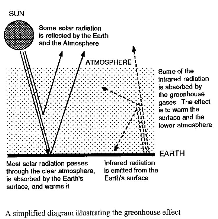
For our detailed reply, please jump up to our diagrams above.
Still, each of the reports misses Houghton's book's (The Physics of Atmospheres, Chapter 2) Equation 2.13, given in all the three editions (1977, 1994, 2002) of the book, shown above, being identical to Goody (1964) Eq. 2.115 (shown above as well, but repeated here):
IPCC WGI (2021) Chapter 8: "Water cycle changes" gives no mention of this equation: that the net radiation at the surface, and the corresponding convective fluxes, are unequivocally constrained to OLR/2 in the clear-sky, and to (OLR – LWCRE)/2 in the all-sky global mean. Further, the latent heat (evaporation) itself, representing the hydrological cycle, is equivalent to 3 units = 80.04 Wm-2, with its best estimate by hydrological cycle assessments as 81 Wm-2, as we have shown here.
Dr. Ramaswamy's current work, Radiative Forcing of Climate (AMS Meteorological Monographs, 2019, Chapter 14), in Fig. 14-1 (page 14.3) shows one early estimate of Earth's global average energy budget, compared with a contemporary estimate of L'Ecuyer et al. (2015), withour realizing that the latter satisfies the net all-sky constraint equation with 0.35 Wm-2 and and the total all-sky constraint equation with a difference of 2.3 Wm-2, as we have shown above and repeat here:
On the same page, in the context of atmospheric radiation transfer, they refer to chapter 2 in Goody and Yung (Atmospheric radiation, Theoretical basis, 1995), without recognizing that Equation (2.146) in that chapter describes the net clear-sky equation in radiative equilibrium [of which the all-sky version is given in our Eq. (3) above]:
L'Ecuyer at al. (2015) is one of the main references of the GEWEX diagram (Stephens et al. 2023, BAMS) which collects the results of 30 years of global energy and water cycle studies, where the two equations are satisfied with an even more extreme, exemplary accuracy of 0.1 Wm-2 (LWCRE is taken from a then-contemopapry study of the same authors):
Ramaswamy, when discussing Manabe's Radiative-Convective Equilibrium model (BAMS 2022), do not realize that the convective adjustment is constrained not only to the net radiation at the surface, but to TOA LW fluxes, thorugh the net all-sky equation (3) shown above.
Ramaswamy, when stating 1.5 - 2.2 Wm-2 radiative forcing from CO2, does not realize that their GFDL Atmospheric Model 4 has exactly the same clear greenhouse effect as the geometric GHG-independent theoretical value, exhibiting no deviation, no enhancement,
suggesting that something else's negative radiative forcing (perhaps water vapor amount decrease or change in its vertical, regional and seasonal distribution) counteracts this positive forcing to maintan the theoretical state required by the constraints.
EVE (Earth Virtualization Engines, Berlin Summit 2023).
We were hesitating on insertig this not-directly science-related material into our list, but as the Max Planck Intitute for Meteorology is involved and Bjorn Stevens (whose energy budget diagram a decade ago triggered the queue of recognitions discussed in this webite) is the second author of the Statement, and, further, as it repeates the typical misunderstandings (or even errors) of the climate consensus, we decided to give two reflextions.
- First, it takes as given a CO2-sensitivity of 2-5 °C as the cause of climate change, without even mentioning detailed LBL-computations resulting in 1 Wm-2 increase of downwardl longwave radiation if CO2 is doubled from 300 to 600 ppm (equivalent to 0.16 °C incrase); and omitting recent understanding that "the global changes observed appear largely from reductions in the amount of sunlight scattered by Earth's atmosphere" (Stephens, Hakuba, Kato et al. Proc. R. Soc. A. 2022).
- Second, it says: " It's really all about the data!", and here we agree !
Norman Loeb in his AGU 2023 Fall Meeting abstract ("Risk and Impact of a Data Gap") says: "Increases
in well-mixed greenhouse gases have led to an imbalance between how
much solar radiant energy is absorbed by Earth and how much thermal
infrared radiation is emitted to space. This
net radiation imbalance, also known as Earth’s energy imbalance (EEI),
has led to increased global mean temperature, sea level rise, increased
heating within the ocean, and melting of snow and sea ice. A recent
study shows that EEI has doubled during the past two decades." Really, in
his October 2023 CERES Science Team Meeting presentation (GISS,
New York) he shows a table on slide #3, with doubling in EEI:
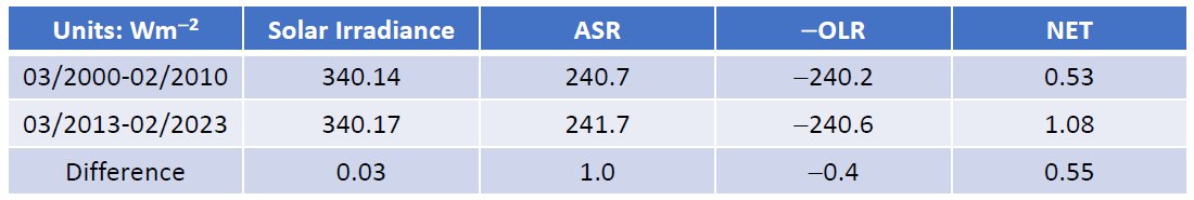
Absorbed solar radiation has been increased by 1 Wm-2, outgoing longwave radiation by 0.4 Wm-2 (the latter is a response to a 0.67 Wm-2 increase in surface Planck-emission). It is evident that EEI has increased because of more solar absorption. There is no established connction between increase in well-mixed GHGs by 20 ppm during this decade (causing 0.08 Wm-2 increase in downward longwave radiation, DLR) and 1 Wm-2 decrease in reflected solar radiation (decrease in cloudiness and / or aerosols). In the prevailing theory, more GHGs are thought to cause a reduction in OLR, not a reduction in albedo.
NOAA says: “Every year we see carbon dioxide levels in our atmosphere increase as a direct result of human activity. Every year, we see the impacts of climate change in the heat waves, droughts, flooding, wildfires and storms happening all around us.”
It is taken as evident that 100 ppm increase in CO2 during the past five or six decades (0.4 Wm-2 increase in DLR, equivalent tp less than 0.1 K° temperature forcing within half a century) might cause those impacts of heat waves or droughts or floodings. — This is exaggregation, even without taken the revealed constraints into acciunt,