| Preface This website offers contemplations we have done in the past ten years. Recent satellite and surface measurement systems are accurate enough to determine the numerical values of the flux elements of the global energy budget with such a precision that allows us to draw quantitative assertions about the ratios and internal relations of these components. First we analyzed two out/in type relationships: - planetary emissivity: the ratio of the longwave radiation leaving the atmosphere at the upper boundary to the longwave radiation entering into the atmosphere at the lower boundary; - infrared transparency: the ratio of longwave radiation at the upper boundary which originates directly from the surface to the surface upward longwave radiation. We then recognized the following characteristics of the basic energy fluxes: — The energy balance equation at the lower boundary (Earth's surface) shows a strong interrelation to the energy balance at the upper boundary (top-of-the-atmosphere); — Most of the observed radiative and non-radiative fluxes are integer multiples of a unit flux, separately for the clear-sky, the cloudy, and the global average (all-sky) fluxes; – Both the planetary emissivity and the infrared transparency have well-defined, prescribed value which can be deduced from a simple model; – The cloud area fraction seems to have an equilibrated (preferred) value, which is constrained to the all-sky planetary emissivity. We collect the basic characteristics of the found pattern in the Foreword and in the Abstract. A Technical foreword collects the players of the global energy budget. We offer some theoretical considerations (conceptual framework) for these results in the Introduction. It begins with some ideas based on the literature; they are then sublimated into questions, then into relationships to be checked on data, forming a model, finally into equations and tables of data, leading to an almost-conclusive deduction of the flux structure; this all is then sublimated into a justifiable forecast. In the History section we survey the evolution of our knowledge of the individual flux components in the energy balance, based on the published global energy budget diagrams. Our Results are compiled into Flux tables and a new Global Energy Budget Diagram and Poster, which you can download and examine in high resolution. Detailed analysis of the individual fluxes in the diagram are given in the Energy flow routes session of the Discussion. We offer also downloadable versions of the Introduction pdf and the Conclusions pdf. Feedback welcome at info@globalenergybudget.com. Miklos ZAGONI
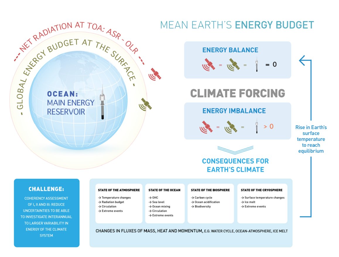
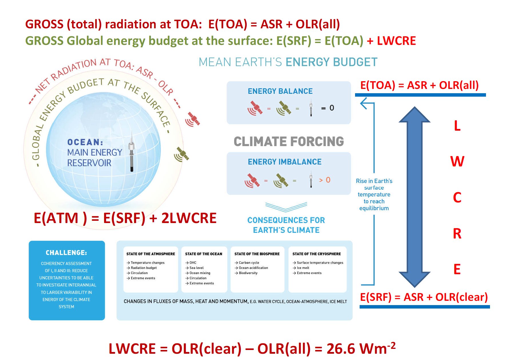
The most important components of the Earth’s global energy budget are: Incoming Solar Radiation (ISR); Reflected Solar Radiation (RSR); their ratio: α = RSR/ISR the planetary albedo; Absorbed Solar Radiation, ASR = ISR – RSR. And further: Outgoing Longwave Radiation (OLR), which in a longer period of time equilibrates to Absorbed Solar Radiation: OLR = ASR. Then Downward Longwave Radiation (DLR), emitted from the atmosphere downward and measured at the surface, called also Back Radiation; and Upward Long Wave (ULW) radiation, emitted by the surface (Planck-, or black-body, or thermal, or infrared radiation). The Absorbed Solar Radiation is partitioned into two portions: one is absorbed by the atmosphere and clouds (Solar Absorbed by Atmosphere, SAA), and the remaining portion which is absorbed by the surface (Solar Absorbed by Surface, SAS; evidently SAA + SAS = ASR). We have also two non-electromagnetic (non-radiative) fluxes from the surface into the atmosphere: Sensible Heating (SH) and Latent Heating (LH), the latter termed also Evaporation (E). Sensible heat is mainly convection, that is, a material current of ascending warm air masses, called also 'thermals', and only a little part of it is heat-conduction. Latent heat release happens by phase change of water vapor into condensed matter; its value, on the global scale, can be evaluated from water cycle analyses. These processes are 'cooling' if looking from a surface perspective. For short, the sum (SH + LH) is often referred to as the 'turbulent' flux. We may insert also the flux components of solar radiation that reaches the surface, Downward Solar Radiation (DSR), and Upward Short Wave (USW) which is reflected from Earth’s land-ocean surface, where the solar absorbed by surface is their difference: SAS = DSR – USW, connected to a surface albedo. And there is a cloud area fraction, β. So we have seven observed flux parameters: three longwave, ULW, OLR and DLR; two shortwave, SAA and SAS, and the turbulent energy flows: SH and LH; and we have two energy balance equations between them: the long-term equilibrium relationship between the absorbed solar and the outgoing longwave radiation at the top of the atmosphere (TOA): E(TOA) = ASR = OLR and the equality of the absorbed (shortwave plus longwave) and the released (radiative plus non-radiative) energy flows at the surface (SRF): E(SRF) = SAS + DLR = ULW + (SH + LH). Hence finally there remains five independent observed flux components. These are the so-called all-sky fluxes, which are observed under global average meteorological conditions in the cloudless and cloudy part of the atmosphere. The ‘fair weather fluxes’ are given separately as clear-sky fluxes. We indicate them as, for example, OLR(all) and OLR(clear), or DLR(all) and DLR(clear). ULW is the only one which is regarded the same in the global annual mean. The cloudy fluxes can be given similarly, for example the annual global mean solar absorbed by surface under clouds is SAS(cloudy). Several composite fluxes can be created as linear combinations of the primary fluxes. We mention here first the difference of clear-sky and all-sky outgoing longwave radiations, OLR(clear) – OLR(all), which is the Cloud Long Wave Radiative Effect, LWCRE: OLR(clear) – OLR(all) = LWCRE. It will play an important role in the followings. * These fluxes are typically described by two parameters: a measured (observed) value, F, and an uncertainty of that observation, given as one standard deviation, ± 1σ. In our study we are going to assign a third parameter to most of them, which we call the F0 value, and will be generated as F0 = I × UNIT. Here I is an integer, and UNIT is a unit flux. In the all-sky case, I is between 1 and 15, and the unit flux is LWCRE, as measured by NASA CERES, and presented in, for example, the updated global energy balance diagram of Stephens et al. (2012) as LWCRE = 26.6 ± 5 W/m2. Our F0(all) values will be one of the following: 26.6 2 x 26.6 = 53.2 3 x 26.6 = 79.8 , … , 14 x 26.6 = 372.4 15 x 26.6 = 399 W/m2. The difference of the observed mean F value and the prescribed F0 = I × 26.6 value is F – F0 = Δ. That is, each of the flux components will be described by a triplet: (F, F0, σ), or, equivalently: (F, Δ, σ). For example, OLR(all) looks like: (239.6, 239.4, ±2) or (239.6, +0.2, ±2). It is evident that such decomposition formally always can be done. But it is meaningful (or useful) only if delta is smaller than sigma; that is, if the proposed F0 values fall into the ±1 sigma range of the observed F value. We will see that this is the case in each examined flux element. In turn, we propose the following F0 values for the above-listed flux elements: F0 = 1 × 26.6 W/m2 for SH, 3 x 26.6 = 79.8 W/m2 for SAA and LH, 6 x 26.6 = 159.6 W/m2 for SAS, 9 x 26.6 = 239.4 W/m2 for OLR, 13 x 26.6 = 345.8 W/m2 for DLR, and, finally, 15 x 26.6 = 399 W/m2 for ULW. We are going to refer to the F0 values as the 'grid position' of the given flux element. In our website we will list the observed F values and their attached 1sigma range from several published studies. They might refer to different observations, satellite and surface measurement systems and networks. Our work is eased by published global energy budget diagrams and tables, where these data are collected and compiled. For example, the latest diagram by Stephens and L’Ecuyer (2015) is based on their own earlier diagram (Stephens et al. 2012), improved by their own energy and hydrological cycle assessments. We are in a comfortable position as we can simply refer to them. There are also well-tabulated data sets as Loeb et al. (2015), and Wild et al. (2015); we will use them too. As said, we can construct important further flux parameters as linear combinations of the above. First of all, the greenhouse effect itself, which is the difference of the surface upward LW radiation and outgoing longwave radiation, separately for the clear-sky and the all-sky case: G(clear) = ULW – OLR(clear) and G(all) = ULW – OLR(all). It is evident that G(clear) = ULW – OLR(clear) = (15 – 10) × 26.6 = 133.0 W/m2, and G(all) = ULW – OLR(all) = (15 – 9) × 26.6 = 159.6 W/m2 It is also evident that G(all) – G(clear) = LWCRE. Further, the difference of surface upward LW radiation and downward LW radiation is called the Net Surface Longwave (NSL) radiation (or net surface radiative cooling): NSL = ULW – DLR, also separately for clear and all-sky. The Longwave Cooling (LWQ) of an atmospheric column is defined as the longwave energy entering from below less that leaving it above and below: LWQ = ULW – OLR – DLR. Evidently, they also have inherited ‘0’ values when they are created from the corresponding F0 value. And there are ‘normalized’ quantities, like g = G/ULW, hence there is also a g0. * There are also non-observable flux components in the system which can only be computed; here one is independent, the longwave radiation in the atmospheric window, which originates from the surface as upward emission and reaches TOA in the mid-infrared ‘window’; called therefore Surface Transmitted Irradiance, STI. Two can be composed: Longwave Atmospheric Absorption: LAA = ULW – STI and a quantity can be called Cooling-To-Space, which is the upward longwave emission from the atmosphere: CTS = OLR – STI; hence the energy balance equation for the atmosphere (ATM), describing the equality of the absorbed (shortwave plus longwave plus non-radiative) energy flows with the emitted longwave energy fluxes: E(ATM) = SAA + SH + LH + LAA = CTS + DLR, see details later. * These are the basic components we are going to deal with in this study. Again, OLR(clear) and DLR(clear) are observed, STI(clear) is computed. We present also these clear-sky values in triplets, assigning an F0(clear) to them as F0(clear) = I × UNIT(clear); for example, OLR0(clear) will be 4 x UNIT(clear). Our results in this website are given in flux numerical tables, and also compiled into a new global energy budget diagram and poster. If you are
interested in some preliminary theoretical
considerations, to set the context, read the Introduction; if
not,
just jump to
the Results – or even to the Summary. Abstract
" Out of love for the truth and from desire to elucidate it, Miklós Zágoni intends to defend the following statements and to dispute on them in that place. Here are my 95 theses. "Introduction We
examine the provocative question:
Are global average radiative and non-radiative flux components in the Earth's atmosphere constrained and quantized? Content of the Introduction:
I. A conceptual framework 1. § "Global warming" is the consequence of more infrared absorption in the atmosphere by more CO2. More absorption means less escaping surface emission in the "atmospheric window". Recent longwave radiative transfer computations clearly show the role of these atmospheric infrared-absorbing gases: When the so-called water vapor continuum is included in the computation, the longwave emission reaching to top of the atmosphere from the surface through the mid-infrared window of the cloudless atmosphere, in global and annual mean, is 66 W/m2; and it is 99 W/m2 when the continuum is excluded. This is the numerical result of Costa and Shine (2012); they use the term "surface transmitted irradiance", STI, for the atmospheric window radiation. Clouds are not transparent in the infrared, therefore the global average "all-sky" radiation in the window is STI(all) = STI(clear) × (1 – β); having the real case with the water vapor continuum absorption and with the observed cloud area fraction of β ~ 60%, we have for the all-sky atmospheric window radiation a value of STI(all) = 26.4 W/m2. With this, they updated the result of Kiehl and Trenberth (1997) (which served the basis for the 2001 and 2007 IPCC reports), who used 99 W/m2 clear-sky and 40 W/m2 all-sky atmospheric window radiation in their famous diagram; Trenberth and Fasullo (2012), and all other energy budget studies published later accepted this update: 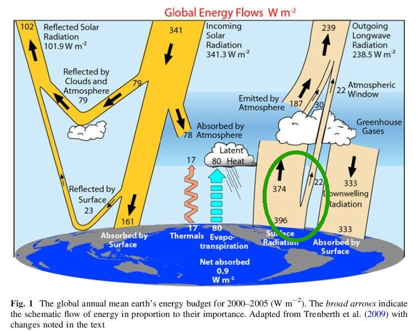 Trenberth and Fasullo (2012) Fig. 1, with the original figure legend. 374 W/m2 is absorbed by the atmosphere and clouds from 396 W/m2 upward longwave surface radiation, and only 22 W/m2 escapes to space through the atmospheric window. Costa and Shine (2012) note about their result that about "one-tenth of the OLR originates directly from the surface". We can add: this also means that only one-fifteenth of the surface emission can get through the atmosphere in the window without being absorbed, since the upward longwave (ULW) emission from the surface is about 398 W/m2. Data uncertainties are about ± 5 W/m2. (TF2012 use 22 W/m2 for all-sky atmospheric window, based on a slightly higher cloud area fraction from an earlier data set. We will examine this question later in detail.) Our atmosphere is really not very transparent in the infrared; where there are clouds, it is effectively opaque, and where are no clouds, it is still rather close to be opaque. For the terrestrial upward
longwave radiation,
the Earth's atmosphere is partially transparent, but it is not too far from being entirely closed. In the all-sky mean, 94 % of the surface longwave emission is absorbed by the greenhouse gases (H2O, CO2, CH4, ozone etc.), and only 6 % gets through and reaches the top-of-the-atmosphere (TOA) in the 'window'. If there is more CO2 (or H2O or methane) in the air, the longwave absorption will increase, hence the surface transmitted longwave irradiance is expected to decrease: the window becomes even tighter, so our atmosphere becomes even less infrared-transparent. This is the best explanation science can offer today: we should take care of the window, we must keep it open. If this is so, the concerns about the increasing atmospheric CO2-content should be taken seriously. *
But.*
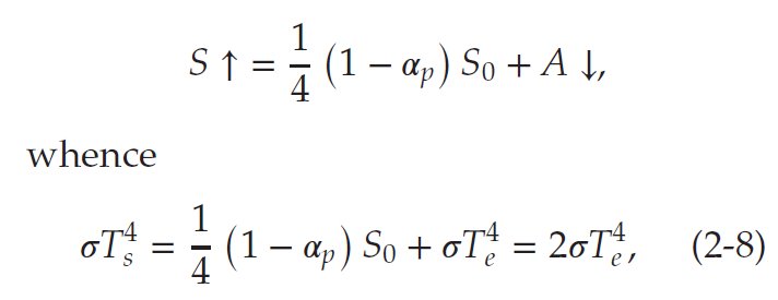
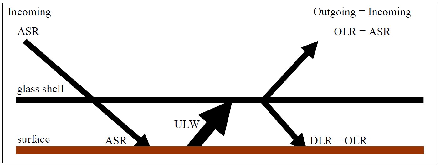
The gap between the 'closed' model and the actual situation of Earth's atmosphere is so narrow that the following approach does not seem implausible: just for curiosity, let us try to understand this '94 % closed' atmosphere from the 'end of the road', when the gap is completely filled; when the whole spectrum of the terrestrial emission is covered; that is, when 100 % of the upward longwave surface radiation is blocked by the atmosphere and 0 % is transmitted from the surface to space (STI = 0). This imagined state can easily be treated by a simple greenhouse model of a planet closed into a 'glass-shell'. A basic textbook example for this case is Figure 2.7 from John Marshall and Alan Plumb: Atmosphere, Oceans and Climate Dynamics, Elsevier 2008, Chapter 2: The global energy balance. Here it is assumed that all the incoming solar radiation gets through the atmosphere and reaches the surface (that is, the 'shell' is completely transparent in the shortwave); and all the longwave surface emission is absorbed by the atmosphere (that is, the shell is 100 % opaque in the longwave). It is also assumed that no turbulent heat is transferred from the surface to the atmosphere: sensible and latent heating (SH and LH) are zero. 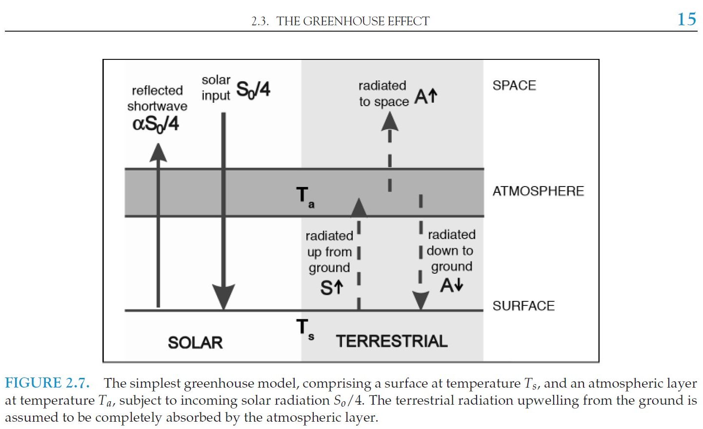 A
single-layer SW-transparent, LW-opaque,
non-turbulent 'glass-shell' greenhouse model. At the surface the energy balance equation is given in Marshall and Plumb Eq. (2-8):
In
our notation system: Absorbed Solar Radiation (ASR) + Downwelling Longwave Radiation (DLR) is balanced by the Upwelling Long Wave (ULW) terrestrial emission: ULW = ASR + DLR. This 'glass shell atmosphere' is assumed to be entirely transparent to the solar flux, but absorbs the longwave upward radiation from the ground completely. As a single-layer shell, it will then radiate the absorbed energy upward and downward equally: OLR = DLR The constraint here is that in equilibrium the Absorbed Solar Radiation is balanced by the Outgoing Longwave Radiation (OLR): ASR = OLR Therefore the surface energy balance equation for the glass-shell model, simply from geometrical reasoning, is: E(SRF) = ULW = ASR + DLR = 2OLR.
The greenhouse effect, defined as surface upward longwave radiation (ULW) less outgoing longwave radiation (OLR), G = ULW – OLR is
then equal to OLR in this model; therefore the normalized greenhouse
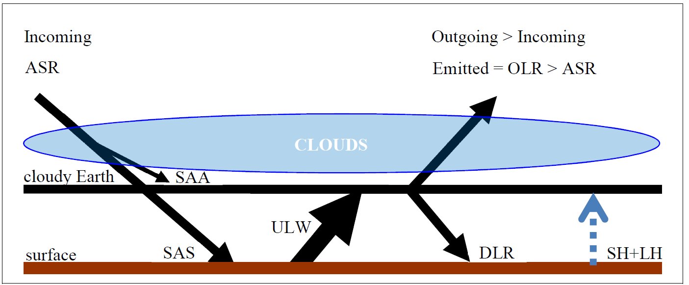
function, g = G/ULW is also equal to * How does this all looks like on Earth? Here the case is different. Our atmosphere is only partially transparent to the solar flux: Solar Absorbed by Atmosphere (SAA) is not zero, therefore Solar Absorbed by Surface (SAS) is less than the total solar absorption: SAS = ASR – SAA. Also, our atmosphere is leaky, that is, only partially opaque to the terrestrial flux, as we have seen above.
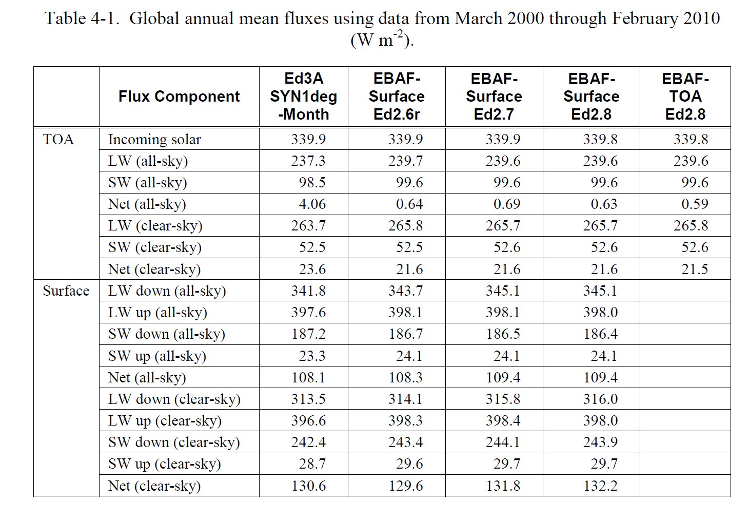
Solar Absorbed Surface (clear-sky), SAS(clear) = Surface SW down (clear-sky) – SW up (clear-sky) = 243.9 – 29.7 = 214.2 W/m2 DLR(clear) = LW down (clear-sky) = 316.0 W/m2 OLR(clear) = TOA LW (clear-sky) = 265.7 W/m2 E(SRF, clear) = SAS(clear) + DLR(clear) = 214.2 + 316.0 = 530.2 W/m2. Compare it to 2OLR : 2OLR(clear) = 2 × 265.7 = 531.4 W/m2. Now THAT is a surprise! The same 'closed model' works in the clear-sky part of the Earth's atmosphere as in the glass-shell geometry! The difference is only 1.2 W/m2, less than half of the error of observation (from ±3 to ±7 W/m2):
This is one of our essential results.
II. Checking the model the on all-sky CERES data 2. §. Citing again NASA CERES data from the table above: SAS(all) = SW down – SW up = 186.4 – 24.1 = 162.3 W/m2 DLR(all) = 345.1 W/m2 OLR(all) = 239.6 W/m2 E(SRF, all) = SAS(all) + DLR(all) = 507.4 W/m2. To compare it with 2OLR(all), the difference is +28.2 W/m2, and to compare it with 2OLR(clear), the difference is -24.2 W/m2. These values are similar to what is lost in the all-sky atmospheric window — far within to the measurement uncertainties. Let us accept for a moment, at least numerically, that E(SRF, all) =
2OLR(clear) – STI(all).
Now THIS relationship would be intelligible. It would mean that: The
Earth's
all-sky atmosphere works like an LW-opaque closed shell,
except one-fifteenth of the surface irradiance, which is escaping to space through the all-sky atmospheric window. As
Marshall and Plumb (2008) show in the model:
 To close our atmosphere in the LW, only 6 % of the surface black-body radiation must be grabbed at. *** Here another quantity will be taken into account: the difference of clear-sky and all-sky outgoing radiations, OLR(clear) – OLR(all), called the Long Wave Cloud Radiative Effect, LWCRE; it is known also as the 'blanketing effect' of the clouds (in contrast to their shielding effect in the shortwave). According to the CERES EBAF Ed2.8 data again: OLR(clear) – OLR(all) = LWCRE = 26.2 ± 3 W/m2. Stevens and Schwartz (2012) refer to this quantity as 26.5 W/m2; Stephens et al. (2012) as 26.7 ± 4 W/m2. CERES DQS says: "LW CRE is determined from the difference between clear-sky and all-sky TOA fluxes." "A marked trend of -0.6 W m-2 per decade is observed in LW Cloud Radiative Effect (CRE) between March 2000 and February 2013. The CERES team suspects at least part of this trend is spurious." Let us keep ourself here to 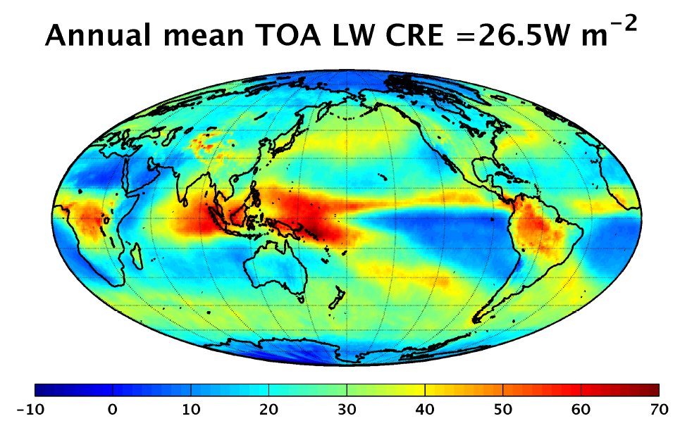 Compare it to the atmospheric window value: Window radiation is STI(all) = 26.4W m–2 From here an idea arises. Could we state that: the longwave radiative effect of clouds is the same as the all-sky atmospheric window? Could we state that the role of the
partial cloud cover in the longwave is
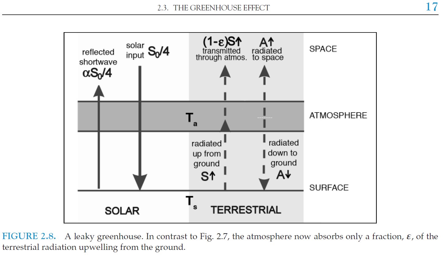
TO CLOSE THE HOLE? TO CLOSE THE WINDOW? This would explain the similar behavior of a closed shell model and the (seemingly) open atmospheric model of the partially cloud-covered Earth as shown in our two figures below: Figure 1. Schematic view representing the concept of a 'leaky' atmosphere. Surface transmitted irradiance, STI(all) is lost in space through the open mid-infrared atmospheric window. Figure 2. Schematic view representing the concept that the all-sky atmospheric window is being closed by the longwave cloud radiative effect, LWCRE. 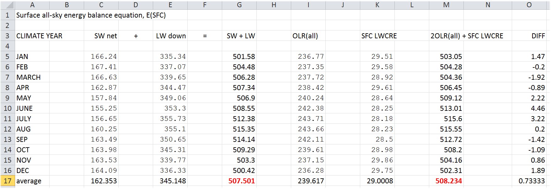 E(SRF, all) = SW net + LW down = 2OLR(all) + LWCRE III. Deduction of the surface energy budget 3.§ Glass-shell geometry, energy budget at the surface: Energy (SRF) = 2OLR Clear-sky
case of
Earth:
Energy (SRF, Earth, clear) = 2OLR(clear) All-sky
case of Earth:
Energy (SRF, Earth, all) = = 2OLR(clear) – STI(all) = 2OLR(all) + LWCRE. It can be written also as = OLR(all) + OLR(clear). This is our result for the energy balance at the Earth's surface; it rests on the measured, published data. A physical explanation can be offered like this: The surface flux being lost in the all-sky atmospheric window STI(all) is gained back by the longwave cloud radiative effect LWCRE. * It is evident that there are a lot of differences between the shell-model and the Earth. For example, Downward longwave radiation is not equal to outgoing longwave radiation: DLR ≠ OLR; There is solar absorption in the atmosphere: SAA ≠ 0, therefore SAS ≠ ASR; and the turbulent heat does not zero: SH + LH ≠ 0. Further, in the clear-sky Earth, the absorbed solar radiation is not equal to the outgoing radiation: ASR(clear) ≠ OLR(clear). But, as we have seen, the clear-sky window radiation is 66.5 W/m2. This means that the atmospheric upward emission (cooling-to-space, CTS) in the clear-sky atmosphere is 266 - 66.5 = 199.5 W/m2, where 266 W/m2 is the clear-sky outgoing LW radiation, OLR(clear). That is, the ratio of the atmospheric upward radiation and surface LW radiation is 199.5 / 399 = 1/2, the same is in the closed model: ULW = 2CTS(clear). The atmospheric layer that radiates directly to space behaves the same way as a closed shell. Further, adding the turbulent fluxes to the surface emission, we have the total surface energy flows as E(SRF, clear) = ULW + (SH + LH)(clear) = 2OLR(clear). This means that (SH + LH)(clear) = G(clear) Data from CERES Table 4.1 last row: Surface net clear-sky: 132.2 W/m2; G(clear-sky) = ULW - OLR(clear-sky) = 398.0 - 265.8 W/m2 = 132.2 W/m2. Therefore E(SRF, clear) = ULW + G(clear) = 2OLR(clear). This also means that 2G(clear) = OLR(clear) THE CLEAR-SKY GREENHOUSE EFFECT IS UNEQUIVOCALLY PREDETERMINED BY OLR(CLEAR). Contrary to all of the internal differences, the logic works:
Later we will see that, according to the data, the same is true for the cloudy part of the atmosphere as E(SRF, cloudy) = OLR(cloudy) + OLR(clear) = 2OLR(cloudy) + LWCRF/beta and ULW = 2OLR(cloudy) - LWCRE/beta. In the all-sky mean: E(SRF, all) = OLR(all) + OLR(clear) = 2OLR(all) + LWCRE and ULW = 2CTS(all) - LWCRE = 2CTS(atm) + LWCRE. Absorbed solar is more than outgoing longwave radiation in the clear-sky part, and there is evident latent heat exchange between the clear and cloudy regions. Still, the whole system maintains the "closed shell" geometry. OLR(clear) = 2G(clear) is equivalent to OLR(clear) = 2(ULW - OLR(clear)), from where arithmetically follows that 3OLR(clear) = 2ULW. Defining the clear-sky transfer function as f(clear) = OLR(clear)/ULW, we have for the closed-shell case: f(clear) = 2/3. With the detailed CERES data: * CERES DATA TABLES 2001 Jan - 2015 Dec: ULW: 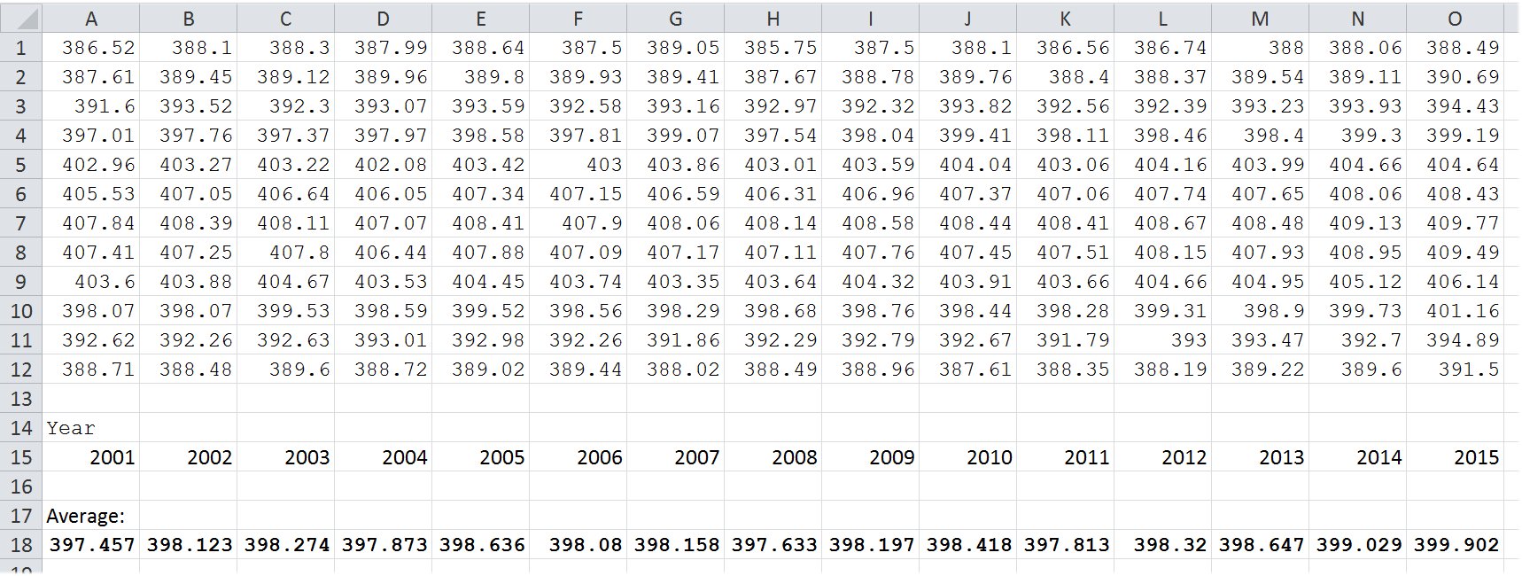 OLR ALL-SKY AND TRANSFER FUNCTION: 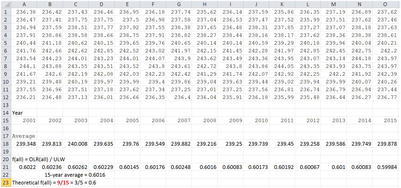 OLR CLEAR-SKY AND TRANSFER FUNCTION: * Though this be madness, yet there is method in't. * Let's see some logical consequences of this geometry: are they valid in the observations? It
can be anticipated that the fluxes
exhibit a wave-like, periodic character, with 'wave numbers' which are integer multiples of a unit flux
of
LWCRE, when propagating in the 'box' between the two
boundaries; like
in the animation below:
 Left
border: Lower boundary (surface)
Right border: Upper boundary (TOA, closed by LWCRE = STI(all)) (Animation is from Wikipedia: https://en.wikipedia.org/wiki/Particle_in_a_box) IV.
Checking the model on the latest published energy budget diagram
We
check the fluxes from the latest published global energy balance
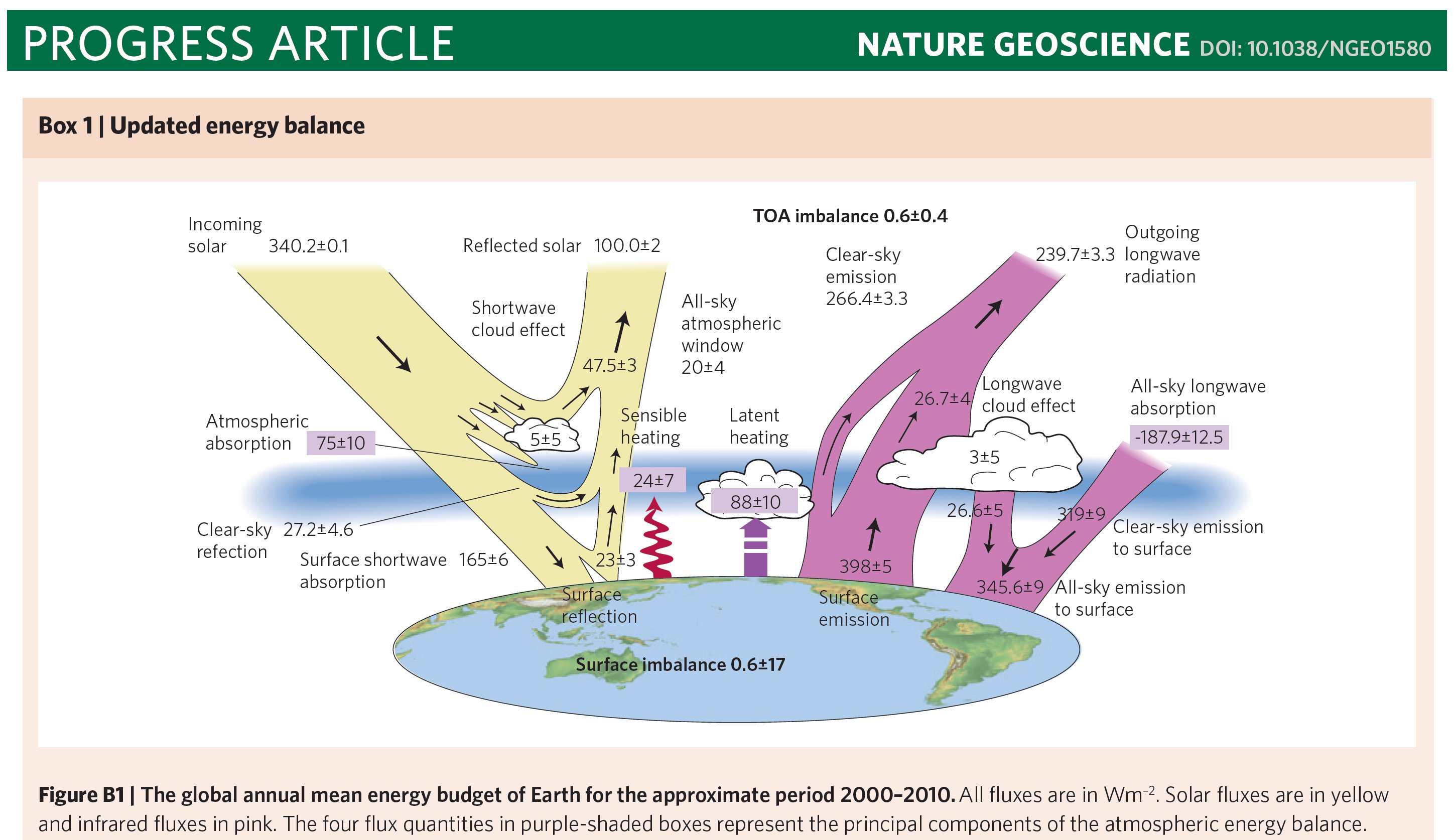
diagram: 4. § Stephens and L'Ecuyer (2015): The Earth's energy balance (Atmospheric Research 166: 195–203) 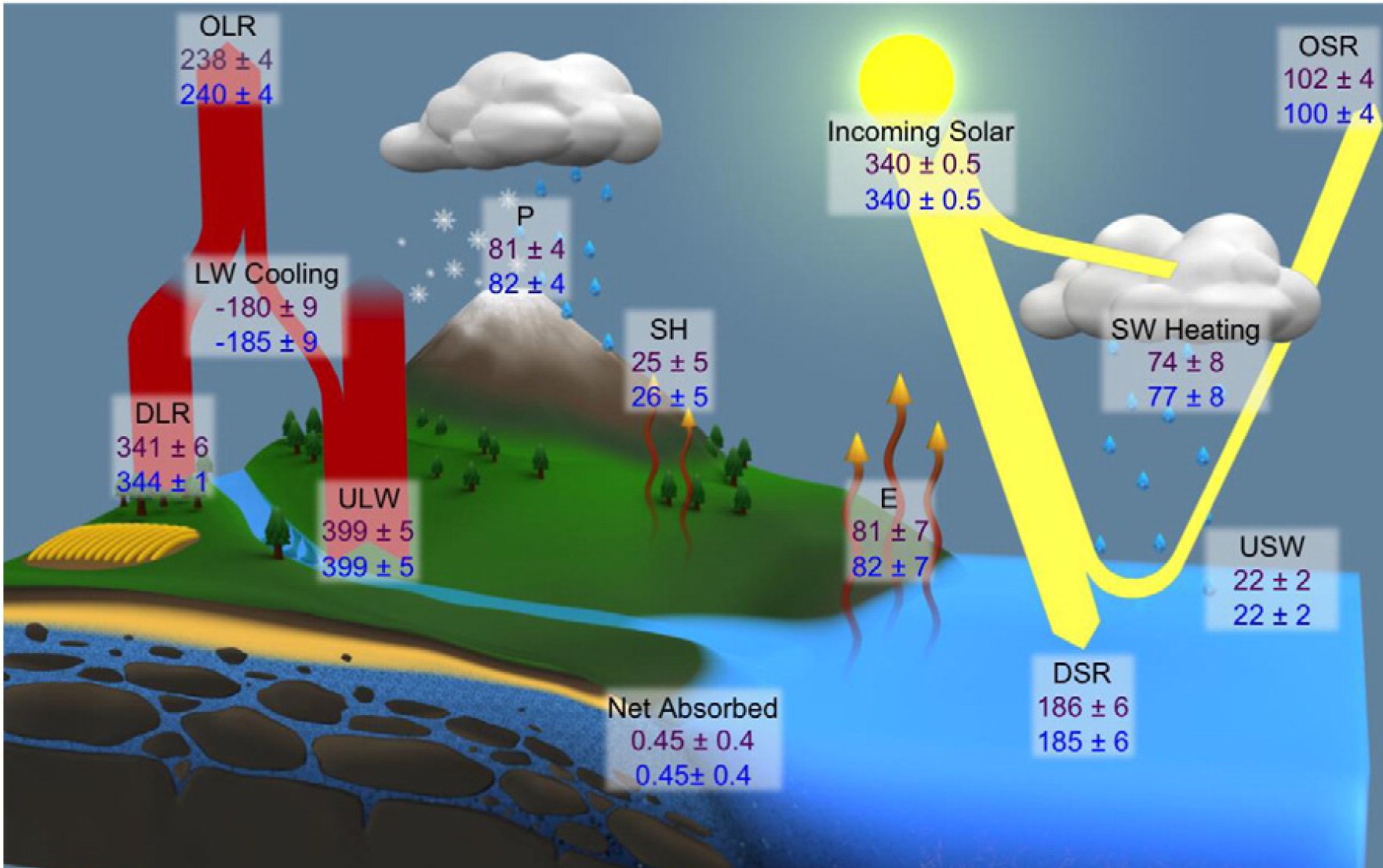 An important energy flow component, clear-sky outgoing radiation, OLR(clear) is not displayed here, but we recall the earlier published energy balance diagram by the same authors (Stephens et al. 2012: An update on Earth's energy balance in light of the latest observations, Nature Geoscience 5: 691-696), where the quantity is presented as: OLR(clear) (Clear-sky emission) = 266.4 ± 3.3 W/m2 Another fundamental components presented in the Stephens et al. (2012) diagram are cloud longwave effect at top-of-atmosphere and at surface: LWCRE (TOA) = 26.7 ± 4 W/m2 LWCRE (SRF) = 26.6 ± 5 W/m2 We
can see that the following F flux mean values
in the diagram are
INTEGER MULTIPLES OF LWCRE (the relative uncertainty and the difference is also shown):
Each of these values appear well within the respective uncertainty range; the only exception is DLR, but the displayed ±1 W/m2 uncertainty in this figure seems too narrow (in the 2012 diagram of the same authors a more realistic error range of ± 9 W/m2 was attached to this quantity; the mean value there was 345.6 W/m2; our 13 × 26.6 = 345.8 W/m2 differs from this only by 0.2 W/m2). Below in this website we examine four publications and prove that the same quantized character appears, with very small differences (Stephens et al. 2012, Stevens and Schwartz 2012, Wild et al. 2015 and Loeb et al. 2015). Further quantities can be constructed as linear combinations of the above: OLR(clear) = OLR + LWCRE is the clear-sky outgoing longwave radiation; NSL = ULW – DLR is Net Surface Longwave cooling; G(clear) = ULW – OLR(clear), and G(all) = ULW – OLR(all) are the clear-sky and all-sky greenhouse effects. Consequently, these flux components have also inherited multiple values as: OLR(clear) = 10 × 26.6 W/m2, NSL = 2 × 26.6 W/m2, G(clear) = 5 × 26.6 W/m2, and G(all) = 6 × 26.6 W/m2. 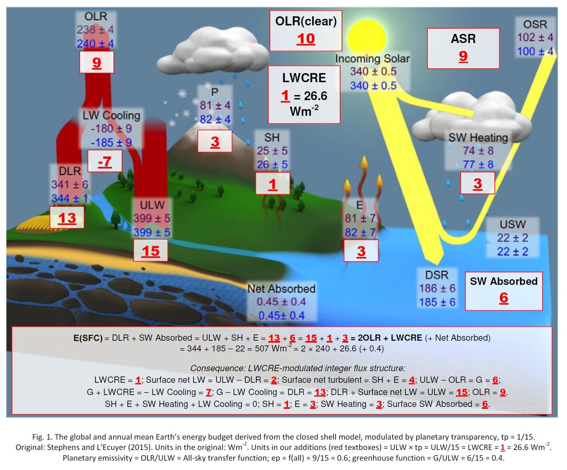 *** So far we were talking about the observable flux components of the global energy budget. But will the non-observable flux components like atmospheric window radiation, which can only be computed, fit into this whole-number structure? From the most recent independent detailed line-by-line computation on realistic atmospheric profiles presents, a result of STI(clear) = 66 W/m2 was published (Costa and Shine 2012). NASA CERES satellite observations show a total cloud area fraction of β ~ 0.605 for the past seven years. For an IR-opaque single-layer effective cloud area fraction we use β = 0.6. The resulted all-sky window radiation is then STI(all) = (1 – β) × STI(clear) = 0.4 × 66 = 26.4 W/m2. If we used the observed mean value of β ~ 0.605, we would have STI(all) = 0.395 × 66 = 26.1 W/m2. Remember, these values are from CERES data; the CERES LWCRE was 26.2 W/m2. Our supposed LWCRE
= (1 – β)
× STI(clear) = STI(all)
equality seems working well. So we accept STI(all) as a further independent element in the table, with a value of STI(all) = 1 × LWCRE, and with a deviation of about ± 0.5 W/m2 or less. Using STI(all), we create two more important flux components as linear combinations of others: atmospheric upward longwave emission (also called Cooling To Space, CTS); for clear and all-sky conditions is defined as: CTS(clear) = OLR(clear) – STI(clear), CTS(all) = OLR(all) – STI(all). Separating the cloud effect from the latter, CTS(atm) = OLR(all) – STI(all) – LWCRE. Assuming that STI(all) = 1, these components in turn will be: CTS(all) = 8, and CTS(atm) = 7. Finally, for clear and all-sky conditions, the portion of surface upward LW emission (ULW) which is absorbed in the atmosphere is the Longwave Atmospheric Absorption (LAA). LAA(all) = ULW – STI(all) = 14. Summarizing these all observable and non-observable fluxes into a table, they form an arithmetic sequence with a common difference of LWCRE:
all within about ΔF = ±3 W/m2 (see the detailed tables with the uncertainties and deviations later). Now the F radiative and non-radiative, observable and only-computable energy flows in Earth's surface and atmosphere seem to follow the "wave-in-a-box" model: they are integer multiples (I) of a unit flux of LWCRE: F = I × LWCRE + ΔF
*
The
observed cloud area fraction, beta is very close to the planetary
emissivity (defined as the ratio between outgoing LW radiation,
OLR(all) and surface upward LW
radiation, ULW, see e.g Bengtsson 2012), called
also all-sky transfer function, f(all).
Again, with the F0 quantities,β = OLR(all) / ULW = f(all) = 9/15 = 0.6. Formally, the all-sky transfer function f(all) is equal to (1 – g(all)), where g(all) is the normalized all-sky greenhouse function, defined as g(all) = G(all)/ULW = (ULW – OLR(all)) / ULW = 6/15 = 0.4. Consequently, the cloudless area of the surface, (1 – β), would be numerically equal to the all-sky greenhouse function g(all). Remember: both the planetary emissivity (transfer function) and the greenhouse function of the closed-shell model were 0.5. On Earth, where one-tenth of the clear-sky emission is a 'lost-in-space' surface radiation through the open all-sky atmospheric window, we are not surprised to have f(all) = 5/10 + 1/10 = 0.6 g(all) = 5/10 – 1/10 = 0.4 The sharp values of these quantities are extremely implausible, unless some planetary-level determinations work in the physical background — or in the geometry. We should regard them annual global mean 'preferred' values, around which oscillations (vibrations, fluctuations, natural or triggered variations) are possible — unknown in size and time-scale. But according to the above-cited, observed and published data, these equalities stand very precisely — at least far within to the accuracy of the observations. This forces us to take our box model seriously. *
For
a little break, notice the following fractions:
G(all)
/ OLR(all) / ULW = 6
/ 9
/ 15
= 2 / 3 / 5
and G(clear) / OLR(clear) / ULW = 5 / 10 / 15 = 1 / 2 / 3. Later we will see that the clear-sky fluxes can be expressed also in clear-sky units as: G(clear)
/ OLR(clear) / ULW = 2
/ 4
/ 6
= 1 / 2 / 3,
where
the clear-sky unit is 1 =
LWCRE / (1 – β)
= 26.6 / 0.4 = 66.5 W/m2.
And there is a cloudy unit as well: 1 = LWCRE / β = 26.6 / 0.6 = 44.33 W/m2 G(cloudy)
/ OLR(cloudy) / ULW = 4
/ 5
/ 9
while
the clear-sky
values in cloudy
units are:
G(clear) / OLR(clear) / ULW = 3 / 6 / 9 This is shown in the top row of our poster (click to enlarge):  A
lot of detailed relationships between the flux elements (like the ratio
of non-radiative to radiative cooling of the surface, and others),
separately for the clear-sky and the cloudy atmosphere, are in several
parts of the Discussion.
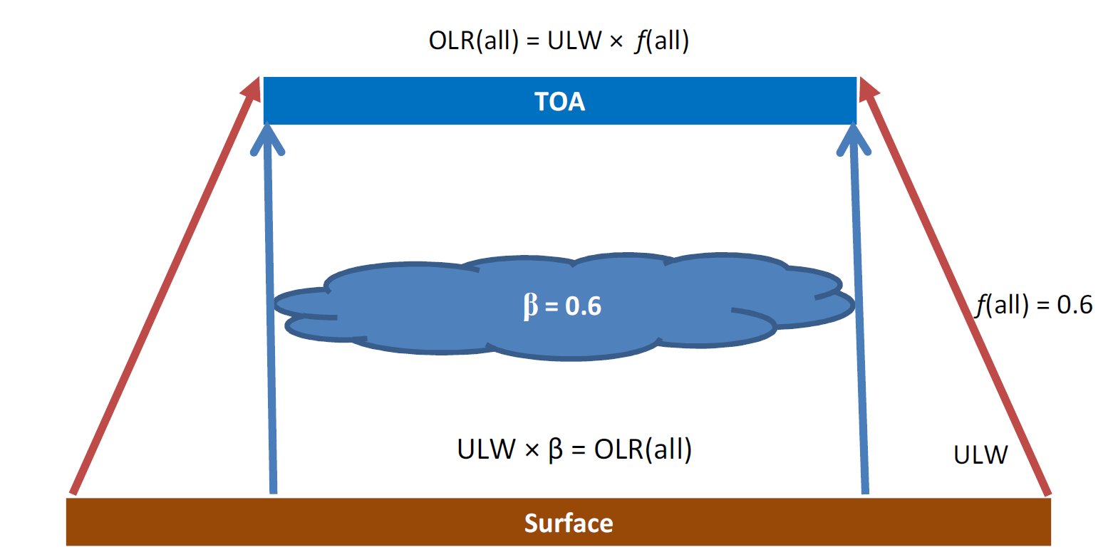
* Several further interesting internal relationships show themselves in the box-model; to mention only one: The
cloud-covered part of the surface, β,
radiates the amount of energy β
× ULW,
which is equal to the all-sky outgoing LW radiation OLR(all): β
× ULW = OLR(all)
*
V.
Checking the energy budget relationship on the latest published diagram5. § Here we point out that the relationship, which connects unequivocally the energy budget of the lower boundary (surface) to the energy flows at the upper boundary (TOA), is THERE in the Stephens and L'Ecuyer (2015) diagram. The surface energy balance equation: Energy (SRF, in) = Solar Absorbed by the Surface + Downward Longwave Radiation = Energy (SRF, out) = Upward Longwave radiative cooling (ULW) and non-radiative (Sensible plus Latent) cooling. With the numbers of the diagram: Energy (SRF, in) = SAS + DLR = 163 + 344 = 507 W/m2 Energy (SRF, out) = ULW + SH + E = 399 + 26 + 82 = 507 W/m2 Note that: Energy (SRF) = 507 W/m2 = 2 × 240 + 26.6 + 0.4 W/m2. Energy
(SRF) = 2OLR + LWCRE
with an imbalance of only 0.4 W/m2, which is also indicated in the diagram (under the name Net Absorbed). If using their LWCRE = 26.7 W/m2, we have 19 × 26.7 W/m2 = 507.3 W/m2; the difference is 0.3 W/m2. The relationship in this diagram is exact — which is intriguing. We can therefore establish E(SRF) as element 19 = 2 × 9 + 1 in our table. According to these data sets, the energy flows at the lower boundary of the box (surface) really appear to equilibrate to the energy flows at the upper boundary (TOA). *** VI.
A quasi-conclusive deduction of the fluxes
6. § Let us survey what we already know about the fluxes in our specific leaky-but-still-closed box model, based on Table II. Number TWO in the E(SRF) = TWO OLR surface energy balance equation of the shell model is an INTEGER, not a well-approximating real number. It is a consequence, a must from the geometry. Also, TWO is an integer is E(SRF, Earth, clear) = TWO OLR(clear). From here, TWO is an inherited integer in the equality TWO CTS(clear) = ULW. It follows that TWO G(clear) = OLR(clear), and TWO STI(clear) = G(clear). In the 'leaky' all-sky mean, we then must have TWO CTS(atm) = LAA(all), which gives, by definition, TWO CTS(atm) = ULW – ONE STI(all); and again by definition, TWO CTS(all) = ULW + LWCRE. The surface energy balance equation is TWO OLR(all) + LWCRE = TWO OLR(clear) – LWCRE = E(SRF, Earth, all), and from here, all the components in E(SRF, Earth, all) will have their INTEGER factor; for example, TWO OLR(all) = ULW + THREE LWCRE, and TWO OLR(clear) = ULW + G(clear). *
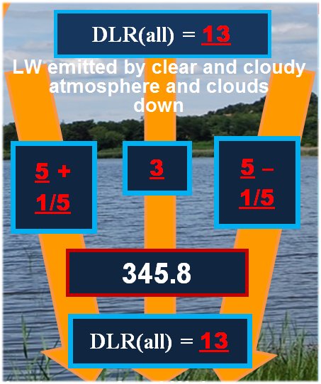
At the upper boundary (top-of-atmosphere, TOA) there are NINE units in the all-sky outgoing radiation, from which EIGHT units are emitted upward from the atmosphere and clouds, and ONE unit is transmitted from the surface. This ONE unit is gained back by ONE unit of longwave cloud effect. At the lower boundary (surface, SRF) there are TWO units of net surface longwave (NSL) radiative cooling and FOUR units of non-radiative cooling (sensible + latent heat release, SH + LH) (with an internal distribution of ONE unit of thermals and THREE units of evaporation). The surface net radiative and non-radiative cooling is then, together, SIX units. These SIX units of surface net and non-radiative cooling are equal to the SIX units of solar radiation absorbed by the surface (SAS), which serves the SIX units of longwave energy content of the greenhouse effect (G). These SIX units of the greenhouse effect, added to net NINE units coming back from the atmosphere, form the FIFTEEN units of gross surface radiative cooling (ULW). This FIFTEEN units of the gross surface radiative cooling, with the FOUR units of surface non-radiative cooling form the NINETEEN units of the total energy release from the surface E(SRF, out) = ULW + (SH + LH). Having FIFTEEN units of surface upward longwave (ULW) radiation and TWO units in net surface longwave (NSL= ULW – DLR) radiation, we must have THIRTEEN units in downward longwave radiation (DLR). This THIRTEEN units in downward longwave radiation, added to the SIX units of solar radiation absorbed by the surface form the NINETEEN units of the total energy income of the surface E(SRF, in) = DLR + SAS. Having FIFTEEN units of surface upward longwave (ULW) radiation and ONE unit in surface transmitted radiation (STI), we must have FOURTEEN units for longwave atmospheric absorption: LAA = ULW – STI. Having FOURTEEN units of longwave atmospheric absorption and SEVEN units in non-longwave atmospheric absorption, we have TWENTY ONE units for the total atmospheric absorption. From these TWENTY ONE units of atmospheric energy income, EIGHT units are emitted upward by the atmosphere and clouds (CTS(all)), and THIRTEEN units are emitted downward to the surface (DLR). This means that SEVEN units are emitted upward by the atmosphere only, and TWELWE units are emitted downward without the cloud longwave effect, leaving TWO units of LWCRE up and down. The TWENTY ONE units in the gross atmospheric energy absorption is then equal to NINETEEN units coming from the surface, plus THREE units coming from solar atmospheric absorption, less ONE unit of surface radiation, as STI is running through the atmosphere without being captured. This TWENTY ONE units in the atmospheric energy content are then equal to NINETEEN units of the gross surface energy content plus ONE up and ONE down longwave cloud radiative effect. This TWENTY ONE units of atmospheric energy content act like a shield of TWO times TEN units of OLR(clear), plus ONE unit of LWCRE. The NINETEEN units of surface energy content is equal to TWO times TEN units of OLR(clear), less ONE unit escaping in the all-sky atmospheric window. The NINETEEN units of surface energy content is equal to TWO times NINE units of OLR(all), plus ONE unit of longwave cloud effect. Having FIFTEEN units of surface upward longwave radiation, NINE units in outgoing longwave radiation and THIRTEEN units in downward longwave radiation, we must have minus SEVEN units in the net atmospheric longwave cooling: LWQ = ULW – OLR – DLR . This minus SEVEN units in the net atmospheric longwave cooling is supplied by SEVEN units of non-longwave atmospheric heating: solar absorbed by atmosphere (THREE units), plus sensible and latent heating (ONE plus THREE units): LWQ + SAA + SH + LH = 0. The SEVEN units of net atmospheric longwave cooling joins to TWO units of net longwave cooling coming from the surface, to form the NINE units of the total thermal cooling of the system: the outgoing longwave radiation. *
NINE units of outgoing longwave radiation and FIFTEEN units of surface upward longwave radiation then define a proper fraction of 9/15 = 0.6 for planetary emissivity, called also transfer function, f(all). SIX units of the greenhouse effect and FIFTEEN units of ULW define a proper fraction of 6/15 = 0.4 for the normalized greenhouse function, g(all). NINE units of outgoing longwave radiation plus ONE unit of longwave cloud radiative effect defines TEN units for the clear-sky outgoing radiation. TEN units of clear-sky outgoing radiation then lead to TWENTY units for the clear-sky surface energy budget, E(SRF, clear) = 2OLR(clear). From this TWENTY units of clear-sky surface energy flows ONE unit is lost in the all-sky mean, leaving NINETEEN units for the all-sky surface energy budget: E(SRF, all) = 2OLR(clear) – STI(all), gained back by ONE unit of the longwave cloud effect: E(SRF, all) = 2OLR(all) + LWCRE. The cooperation between the clear-sky part and the all-sky energetic requirements is created by a partial cloud cover; with a total single-layer IR-opaque effective cloud area fraction β = (NINE units of OLR) / (FIFTEEN units of ULW) = 9/15 = all-sky transfer function = 0.6 = planetary emissivity. *
TEN units of clear-sky outgoing longwave radiation contribute to the all-sky global average with an area-weighted value of (1 – β) × OLR(clear) = FOUR units. Therefore, the cloudy part contributes to the NINE units of all-sky OLR with FIVE units, having a nominal outgoing longwave radiation above clouds OLR(cloudy) = FIVE / β . NINE units of OLR(all) is therefore being partitioned as NINE = OLR(all) = (1 – β) × OLR(clear) + β × OLR(cloudy) = FOUR + FIVE. Hence, the cloudy unit is ONE/β, and the clear-sky unit is ONE / (1 – β). Numerically: ONE = UNIT(all) = OLR(clear) / 10 = 26.6 W/m2, then ONE / β = UNIT(cloudy) = 26.6 / 0.6 = 44.33 W/m2, and ONE / (1 – β) = UNIT(clear) = 26.6 / 0.4 = 66.5 W/m2. The surface energy budget under clouds is given then: E(SRF, cloudy) = 2OLR(cloudy) + UNIT(cloudy) = 2OLR(clear) – UNIT(cloudy). The clear-sky and the cloudy-sky tables will be given later separately; the whole structure is presented in our poster. More details in the Discussion. *** What's happening with the window if there is more CO2 in the air? The latest NASA AIRS instrument has actually measured the decrease in IR energy from the Earth as CO2 in the atmosphere has increased. This is observational evidence that increased CO2 reduces the rate of loss of IR energy to outer space. But we have also observational evidence that the whole flux structure still maintains the integer ratio system and that the greenhouse effect keeps its narrow value at its required position. What's going on? It seems that the overall planetary-level energetic control, which determines the closed-model geometry, poses effective constraints on the entire radiative transfer process, and it can be anticipated that the most powerful greenhouse gas, water vapor could play the leading role, through evaporation, precipitation, cloud formation and greenhouse effect-regulation. The given energy flow structure belongs to a very specific, unique annual global mean vertical temperature distribution. Though one element is perturbed by anthropogenic emissions, all the other elements together seem to be able to act as an effective stabilizing feedback network. *
We do not have enough data to talk about these fluxes and their relationships during transient climatic conditions, under glacial and interglacial circumstances. We can only say what we see: that these identities and integer ratios are there in the data covering the recent decades of accurate satellite observations; some of them are almost exact, and all of them are surprisingly close. It is remarkable that, contrary to the above-referred AIRS observations, the two substantial boundary radiative fluxes, OLR and ULW fit the best: with 0.2 W/m2 and 0.0 W/m2 deviation into the integer structure. We regard this as a strong indication that the box model might be valid. It is to be emphasized also that we are finding ratios and relationships between energy flows, not absolute values of flows: the all-sky unit is relative to OLR(all), the clear-sky unit is relative to OLR(clear). ***
An uneasy note on terminology. When we mention 'quantized', we evidently do not mean the precisity of atomic quantum levels. We just wanted to express that 'not continuously changing'. For example, using the observed and published data from the tables above: as long as OLR(all) = 239.4 W/m2, DLR(all) cannot be, say, 360 W/m2, but must be 345.8 W/m2; and ULW cannot be 408 W/m2, but must be 399 W/m2 — without knowing of course how far and how fast the climate could deviate from, or fluctuate ('vibrate') around, these integer relationships. Originally we tried to use the word 'periodic', and called our tables 'flux periodic tables', in the sense of Merriam-Webster: 'ocurring or recurring at regular intervals'; 'consisting of or containing a series of repeated digits'; periodicity: 'the quality, state or fact of being regularly recurrent'; a near antonym of 'continuous'. A British friend of us supported this notion; but then two of our American friends practically forbade us to use this ("NOT periodic !!!"). Not being a native English speaker, we are lost here. We simply mean that the energy flow 'quantum' is one LWCRE in the closed box, being equal to OLR(clear)/10, and the flux values are integer multiples of this. Use 'pattern', 'wave number', 'arithmetic sequence' or 'progression' if you wish. Physically think of the wavelengh of a wave propagating in a box, or anything that cannot change continuously but exhibits discrete, 'quantized' character. Once we were trying to use the expression: "The global energy flow system has an internal structure." Now that was a big mistake! We were sent books from the UK about 'structures': "What kind of internal structure an atmospheric energy flow might have?!" So we abandoned that idea too... The same with 'constrained'. One of our friends proposed to use this word, another fiercely opposed, and suggested 'equilibrated' instead, like: "The surface energy flows are equilibrated to the energy flows at TOA." This might be correct. We simply mean that, according to the published data: F = I × LWCRE + delta F, where I is an integer, LWCRE = OLR(clear)/10, and the little delta is smaller than the standard deviation σ. and: E(SRF, all) = 2OLR(all) + LWCRE, etc. The take-away message here is this: you are asked to focus on the numbers. They carry our primary message; do not let our immature terminology to distract your attention. ***
So we state three substantial findings here: I. The surface energy budget is constrained to the energy flows at TOA II. There is a discrete pattern in the fluxes III. The above two features can be explained by a specific closed-model analogy. These three, inter-related results give us enough confidence to state the followings: This particular, constrained and quantized characteristic of the atmospheric energy flow system is a completely different paradigm from the prevailing climate theory, which expects increased greenhouse effect from the increased CO2 content of the atmosphere: 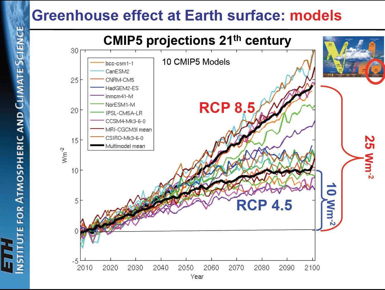 Slide #59 from
the presentation of M. Wild (2015a): Energy Cycles in the
global climate system.
If the above-presented numerical relationships are long-standing and valid and the Earth really maintains the said closed-system character, then this increase in the greenhouse effect cannot happen. Let this justifiable forecast be the bottom line of this Introduction. *** We continue here with a History, where you can find all the published global energy budget diagrams, to track the evolution of our knowledge of the individual energy flow components in the global energy budget. In the Discussion we examine several details of our findings and show numerous internal relationships between the separate clear-sky and cloudy-sky flux components. We try also try to track the energy flow routes through the climate system, where each part of our diagram is discussed. In the Results section we present the clear-sky, the all-sky and the cloudy flux tables; for comparison, a closed model table is also presented. We compile our findings in a new global energy budget diagram, built into a detailed informative energy budget poster, which you can download and examine in high-resolution. Alternatively, you can jump to the Conclusions, or directly to the Summary. Please send your feedback to info@globalenergybudget.com. Enjoy your exploration into this fascinating world of Earth's global energy budget. Miklos ZAGONI  History Earth's Radiation Budget: The First 20 Years Though the golden era of Earth's energy budgets started with the diagram of Kiehl and Trenberth (1997), we still start with a diagram from almost 100 years ago. 7.§.
Dines 1917The first known graphical representation of Earth's global energy budget is from William Henry Dines (1917) The heat balance of the atmosphere. Q. J. R. Meteorol. Soc. 43: 151–158 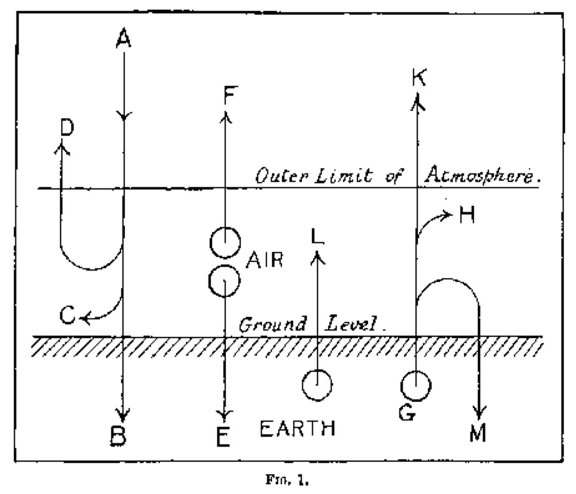 8.§.
Rudolf Geiger 1950Another image is given by Rudolf Geiger: The climate near the ground, 1950, Harvard Univ. Press: 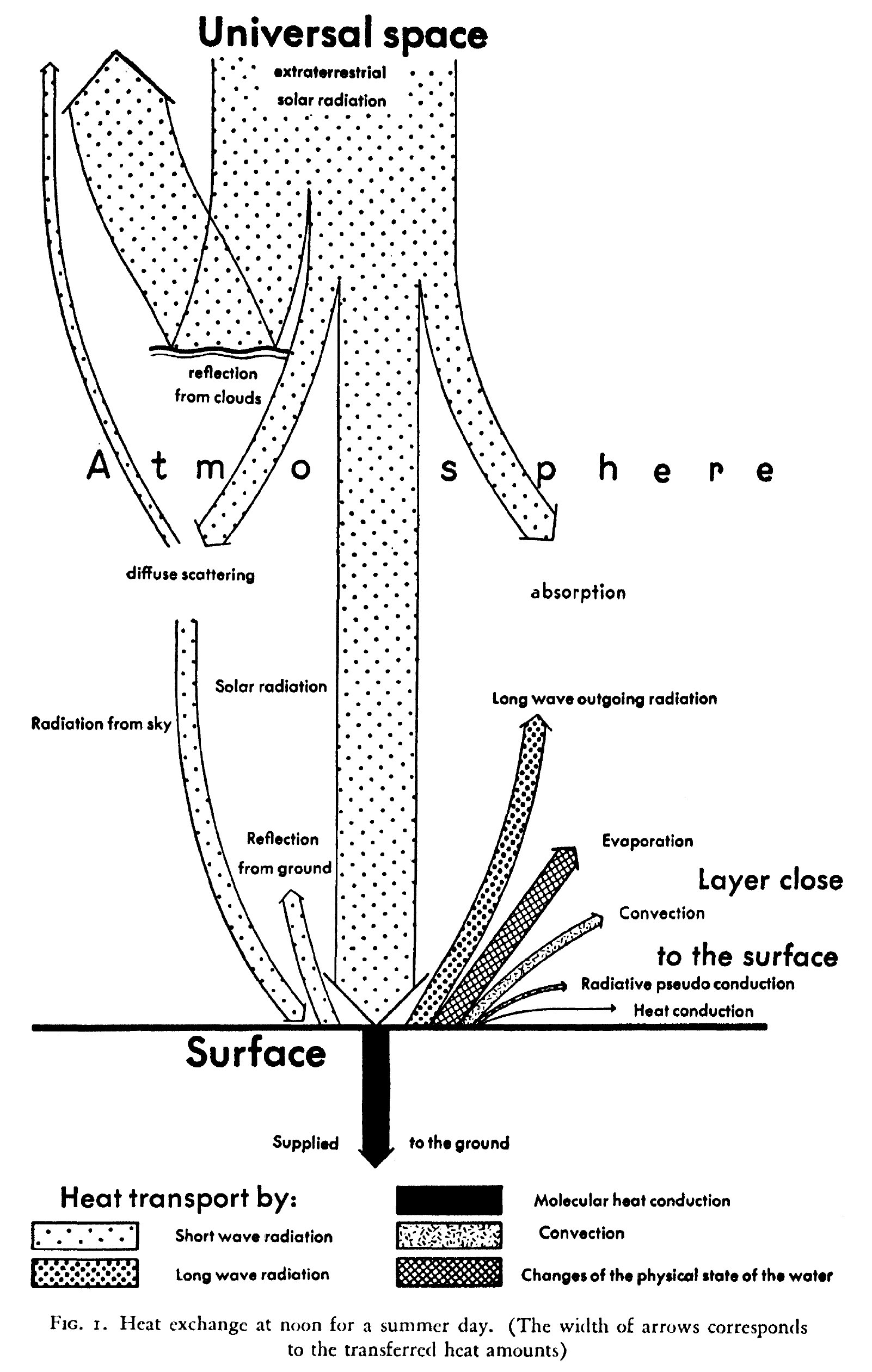 9.§.
Rudolf Czelnai 1979Rudolf Czelnai in his 'Introduction to meteorology' (1979) university lecture notes (in Hungarian) gives good approximations: 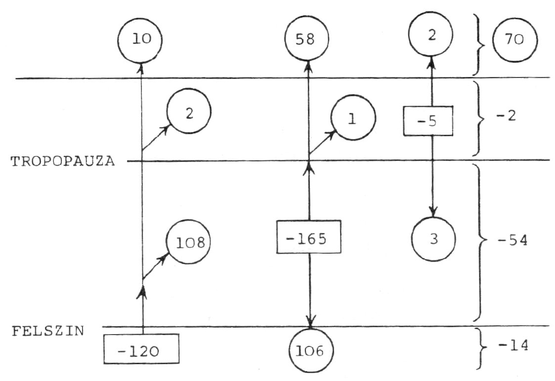
Surface and atmospheric LW budget (%) 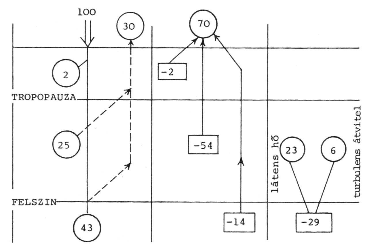 Surface and atmospheric energy budget: SW, LW, latent and sensible (%) TOA fluxes in Cess et al. (1996): Cloud feedback in atmospheric GCM Numbers, they say, have been rounded for the purpose of illustration. 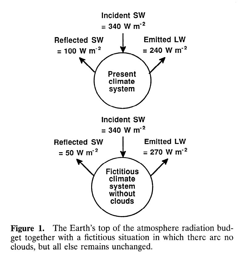 "Because clouds are bright, their presence increases reflection of shortwave (SW) radiation by 50 W/m2 (cooling), while the greenhouse effect of clouds results in a longwave (LW) warming of 30 W/m2." 10.§.
Kiehl
and Trenberth 1997Earth's Annual Global Mean Energy Budget Bull Am Meteor Soc 78:197–208 The original diagram: 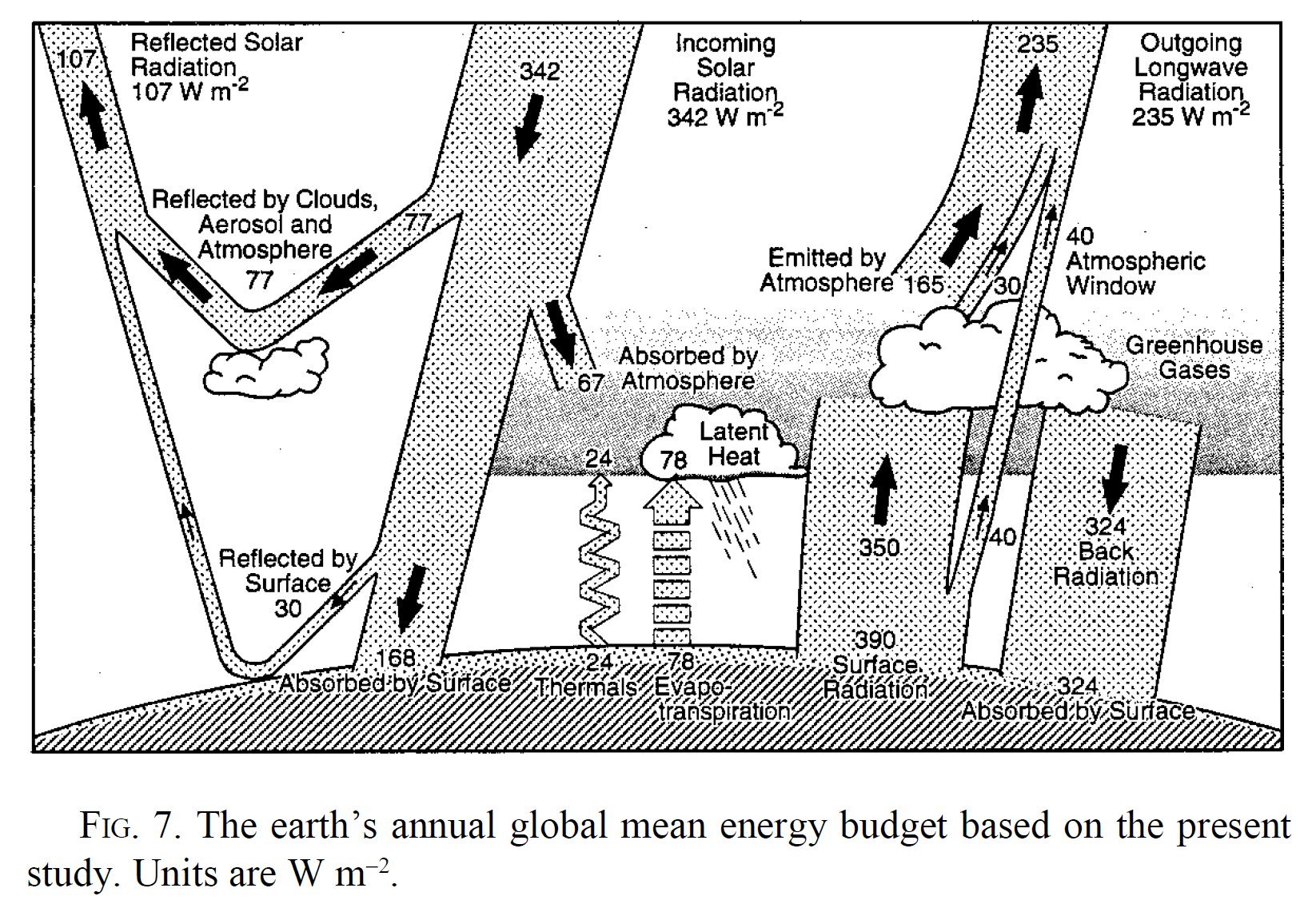 and its spectacular colored version, with the same data, from a NASA website: 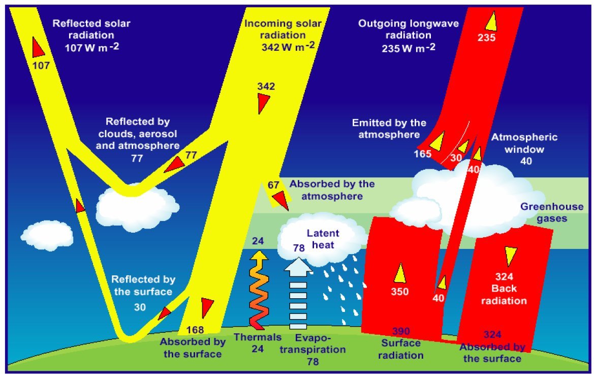 The
top-of-the-atmosphere (TOA) shortwave (SW)
and longwave (LW) flux of energy is from ERBE (Earth
Radiation Budget Experiment) satellite observations (1985-1990).
Fluxes within the atmosphere were computed from detailed radiation models. The surface infared radiation of 390 W/m2 corresponds to a blackbody emission at 15 °C. The radiative greenhouse effect (G) (or as they call, the longwave radiative forcing) is the difference of the upwelling longwave radiative fluxes at the two boundaries, G(all) = Surface Radiation – Outgoing Longwave Radiation(all) = 390 – 235 = 155 W/m2 for the average cloudless-and-cloudy conditions (the so-called 'all-sky' case). The Outgoing Longwave Radiation over the cloudless regions is OLR(clear) = 265 W/m2 (see their Table 2), so the clear-sky greenhouse effect is G(clear) = 390 – 265 = 125 W/m2. The longwave cloud effect is hence LWCF = G(all) – G(clear) = OLR(clear) – OLR(all) = 30 W/m2. The all-sky outgoing longwave radiation of 235 W/m2 is partitioned into 165 W/m2 'Emitted by Atmosphere' + 30 W/m2 'to show the LWCF' + 40 W/m2 'Atmospheric Window'. The latter is the radiation that originates from the Earth's surface and is transmitted relatively unimpeded through the atmosphere. The energy balance equation at the surface is: absorbed shortwave plus longwave energy (168 + 324) = radiative (390) plus non-radiative (24+78) cooling. 'Net' surface longwave cooling: LW up minus LW down = 390 – 324 = 66 W/m2, 'gross' (radiative plus non-radiative) surface cooling: 168 W/m2. The diagram served the basis for the third assessment report of the IPCC in 2001. |
|||||||||||||||||||||||||||||||||||||||||||||||||||||||||||||||||||||||||||||||||||||||||||||||||||||||||||||||||||||||||||||||||||||||||||||||||||||||||||||||||||||||||||||||||||||||||||||||||||||||||||||||||||||||||||||||||||||||||||||||||||||||
11.§.
Wild et al. (1998)The disposition of radiative energy in the global climate system: GCM-calculated versus observational estimates Clim Dyn 14: 853-869 An alternative from 1998: Martin Wild et al., based on direct observations.  Most
important proposed differences:
OLR(clear-sky): 263 W/m2 Cloud radiative forcing, TOA: 28 W/m2 Cloud radiative forcing, surface: 21 W/m2 Back Radiation, all-sky: 344 W/m2 Back Radiation, clear-sky: 323 W/m2 Net surface LW cooling: 53 W/m2. It is
only of
historical interest that the Wild et al. 1998 paper, submitted one year
after the KT97 article appeared in the BAMS 1997 February issue,
proposes sevaral updates without even referring to it.
|
|||||||||||||||||||||||||||||||||||||||||||||||||||||||||||||||||||||||||||||||||||||||||||||||||||||||||||||||||||||||||||||||||||||||||||||||||||||||||||||||||||||||||||||||||||||||||||||||||||||||||||||||||||||||||||||||||||||||||||||||||||||||
12.§.
The diagram in the UN IPCC 2007 Fourth
Assessment Report. It is thought to be identical with the original. But is it? Find the difference! (IPCC WGI AR4 2007 Ch 1 Fig 1) 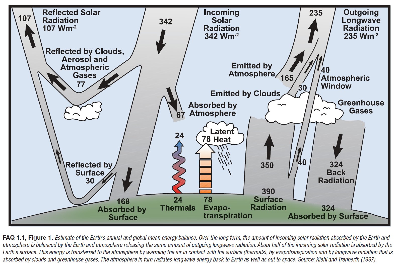 A
new label appears here: 'Emitted by Clouds', attached to the 30 W/m2.
But the KT97 paper states: "The atmospheric emitted radiation is apportioned into two parts to show the LWCF of 30 W/m2". Longwave cloud effect is the reduction of the clear-sky outgoing longwave radiation, 265 W/m2, to the all-sky mean, 235 W/m2, in the presence of clouds; and not an individual additive energy flow component of the all-sky outgoing radiation. And it is far too low to be the real cloud-top emission. KT97 calculate with a ~60% cloud coverage. This means that the 265 W/m2 of outgoing radiation belongs to the ~40% cloudless area, with a contribution to the all-sky mean: 0.4 × 265 W/m2 = 106 W/m2. Hence, from the cloud-covered part of the atmosphere must come the remaining 235 – 106 = 129 W/m2, instead of 30 W/m2. Interestingly, this controversial label appears also in the NASA Earth Energy Budget Poster as well, see later. |
|||||||||||||||||||||||||||||||||||||||||||||||||||||||||||||||||||||||||||||||||||||||||||||||||||||||||||||||||||||||||||||||||||||||||||||||||||||||||||||||||||||||||||||||||||||||||||||||||||||||||||||||||||||||||||||||||||||||||||||||||||||||
13.§. Trenberth,
Fasullo and Kielh (2009)
Earth's Global Energy Budget Bull Am Meteor Soc 90:311–323 The
proposal of Wild et al. (1998) to increase back-radiation (DLR) from
324 W/m2 to 344 W/m2
was only partially accepted by the authors of KT97. 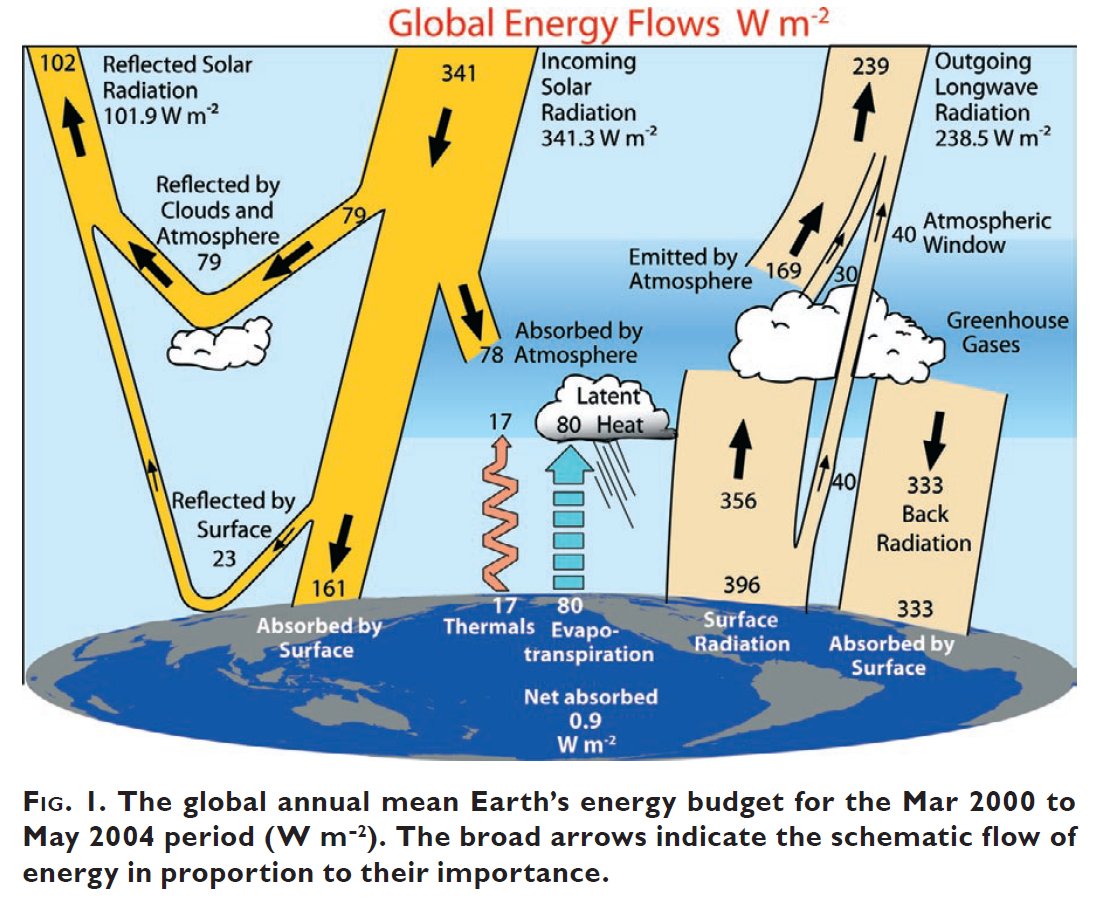 This
is the first update of KT97, based on the newly
available CERES (Clouds and the Earth's Radiant Energy System)
satellite data from 2000 to 2004. The presented changes follow the
proposals of Wild et al. (1998). Shortwave atmospheric absorption (78)
and Back Radiation (333) was increased; surface SW reflection (23) and
absorption (161) decreased; new Surface Radiation (396) and Outgoing
Longwave Radiation (238.5). Window (40) and LW cloud radiative effect
(30) remain unchanged. Greenhouse effect: LWup(surface) – LWup(TOA) =
396 – 238.5 = 157.5 W/m2. Net surface LW cooling: 396 – 333 = 63 W/m2.
A surface net absorption (0.9 W/m2) is first introduced.
*
Funny
enough that "The Atmospheric
Radiation Measurement (ARM) Program: The First 20 Years",
published in 2016, still uses this 2009 diagram as a basic reference,
despite the fact that its authors themselves published an update to it
in 2012, let alone other upgrades from 2013 and 2015. Wrong window
value, wrong atmospheric LW absorption and emission, outdated LWCRE ...*
The graphic really
became famous: The
Economics created its own version (with
the expressive title: The clouds of unknowing. Mar 18th 2010):
|
|||||||||||||||||||||||||||||||||||||||||||||||||||||||||||||||||||||||||||||||||||||||||||||||||||||||||||||||||||||||||||||||||||||||||||||||||||||||||||||||||||||||||||||||||||||||||||||||||||||||||||||||||||||||||||||||||||||||||||||||||||||||
14.§. M.
Wild (2012) Facelift for the picture of global energy balance
Atm Env 55: 366-367 In
2012 Wild asserted again that DLR must be about 344 W/m2, and, as
TFK2009 accepted,
solar absorbed by surface (SAS) must be about 160 W/m2: 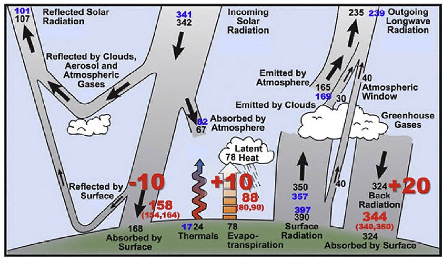 Other
proposed changes are mainly consequences and necessary adjustments
because of this basic change of Back Radiation to 344 W/m2. Very
important: uncertainty estimates (340, 350) also attached. Based on
improved hydrological cycle estimates, the new proposed non-radiative
surface cooling (the sum of the turbulent fluxes: thermals
plus
evaporation) is 17 + 88 =105 W/m2.
|
|||||||||||||||||||||||||||||||||||||||||||||||||||||||||||||||||||||||||||||||||||||||||||||||||||||||||||||||||||||||||||||||||||||||||||||||||||||||||||||||||||||||||||||||||||||||||||||||||||||||||||||||||||||||||||||||||||||||||||||||||||||||
15.§.
Costa and Shine (2012):
Outgoing Longwave Radiation due to Directly Transmitted Surface Emission Costa and Shine (2012) state that the purpose of producing the value is "mostly pedagogical". They seem to be too humble. "Atmospheric Window" is one of the most fundamental quantities: it describes the amount of surface irradiance going through the atmosphere and leaving to space without absorption. If you think of the greenhouse effect as the "heat-trapping capacity" of the atmosphere, then this is the quantity that is not trapped: it measures the infrared transparency (or opacity) of the atmosphere. Its value in KT97 is given as 40 W/m2, as KT97 calculated the clear-sky window radiation to be 99 W/m2, and, regarding a 60% single-layer LW-opaque cloud area fraction, they have 99 × 0.4 ~ 40 W/m2 for the all-sky mean. But Costa and Shine re-calculated this quantity and found that KT97 handled the water vapor continuum incorrectly; their proposed new value for the clear-sky surface transmitted irradiance is STI(clear) = 66 W/m2, instead of 99 W/m2. 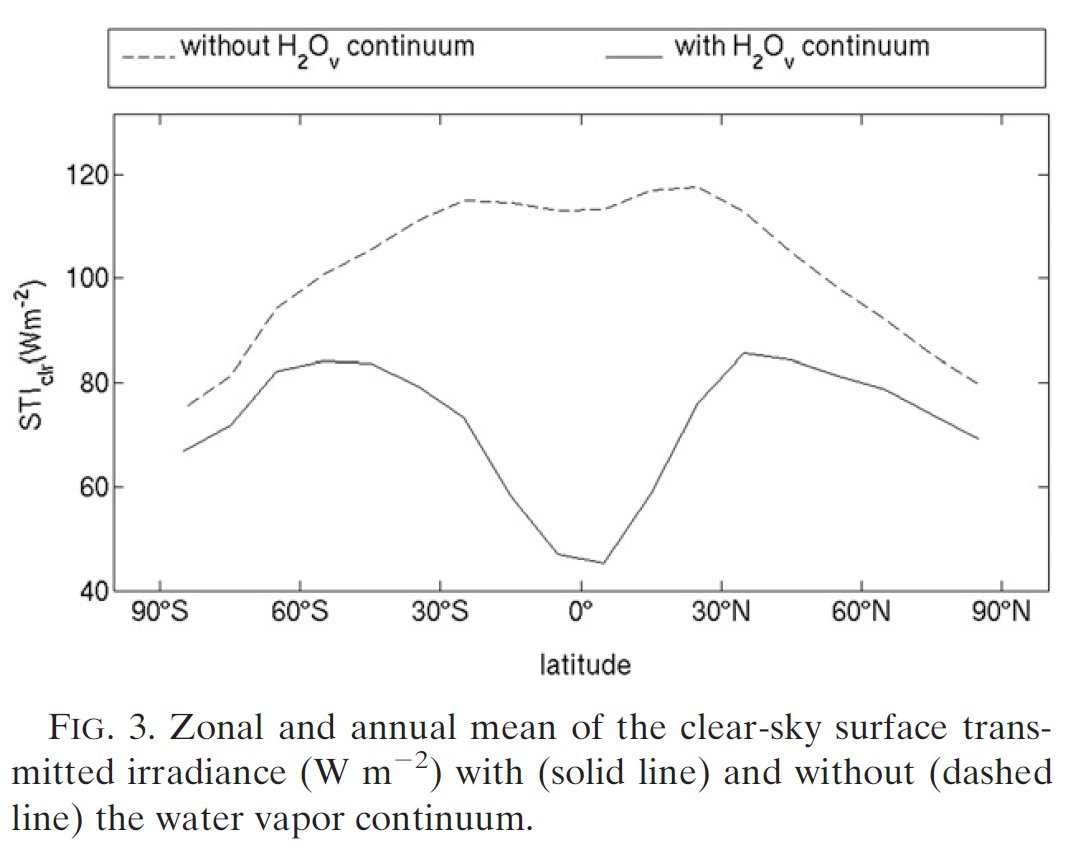 Costa S, Shine K (2012) Outgoing Longwave Radiation due to Directly Transmitted Surface Emission Journal Atmos Sci 69: 1865–1870 |
|||||||||||||||||||||||||||||||||||||||||||||||||||||||||||||||||||||||||||||||||||||||||||||||||||||||||||||||||||||||||||||||||||||||||||||||||||||||||||||||||||||||||||||||||||||||||||||||||||||||||||||||||||||||||||||||||||||||||||||||||||||||
16.§. Trenberth
and Fasullo (2012):
Tracking Earth's Energy: From El Nino to Global Warming Surv Geophys 33: 413–426 Trenberth
and Fasullo (2012) immediately accepted the STI(clear) = 66 W/m2 of
Costa and Shine,
and, having an earlier estimate of cloud area fraction of 67% from ISCCP 1999, they assigned a new value to the all-sky window radiation as 66 × (1 – 0.67) = 22 W/m2 in their new update. As a consequence, LW atmospheric absorption became 396 – 22 = 374 W/m2, and the emitted by atmosphere upward flux element is now 239 – 30 – 22 = 187 W/m2. It can be seen that every value was changed from the original KT 1997 picture, with the only exception of 30 W/m2, assigned to the clouds. 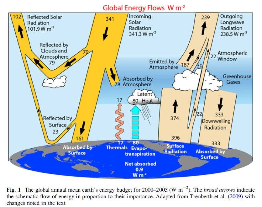 [ I
beg your pardon? The value of an absolutely essential climate
parameter, "Atmospheric Window", describing the atmospheric
transparency, published in the 2001 and 2007 UN IPCC reports, was halved? From
40 W/m2 of KT97 to 22 W/m2 of TF12 ? — Well, yes ... Actually,
the new value is two-thirds of the original (as the new STI(clear) = 66
W/m2 is two-thirds of 99 W/m2 of KT97), assuming the same cloudiness.
Hence, as the original all-sky "Atmospheric Window" was (1 –
0.6)
× 99 W/m2 = 40 W/m2, now its best value is (1
– 0.6) × 66 W/m2 = 26.4 W/m2.
]
|
|||||||||||||||||||||||||||||||||||||||||||||||||||||||||||||||||||||||||||||||||||||||||||||||||||||||||||||||||||||||||||||||||||||||||||||||||||||||||||||||||||||||||||||||||||||||||||||||||||||||||||||||||||||||||||||||||||||||||||||||||||||||
| 17.§. What
is this "30" W/m2 after all, attached to the clouds in all of these
figures?
The UN IPCC 2007 diagram says it is “Emitted by Clouds”. This label is missing from the original KT97 figure. But it cannot be cloud-top emission. If the all-sky outgoing longwave radiation is 239 W/m2, and the clear-sky outgoing radiation is 266 W/m2, then, having a 60% global average annual mean cloudiness, the contribution of the clear-sky part is 266 × 0.4 = 106 W/m2. This leaves 239 – 106=133 W/m2 for the cloudy part. So the value of 30 W/m2 as cloud-top radiation is far too little. |
|||||||||||||||||||||||||||||||||||||||||||||||||||||||||||||||||||||||||||||||||||||||||||||||||||||||||||||||||||||||||||||||||||||||||||||||||||||||||||||||||||||||||||||||||||||||||||||||||||||||||||||||||||||||||||||||||||||||||||||||||||||||
18.§.
Interestingly,
the NASA Langley Center’s Energy Budget Poster from 2014 still contains this description. And, they didn’t bother to change the atmospheric window radiation from the original 40 W/m2 to the newly computed one. 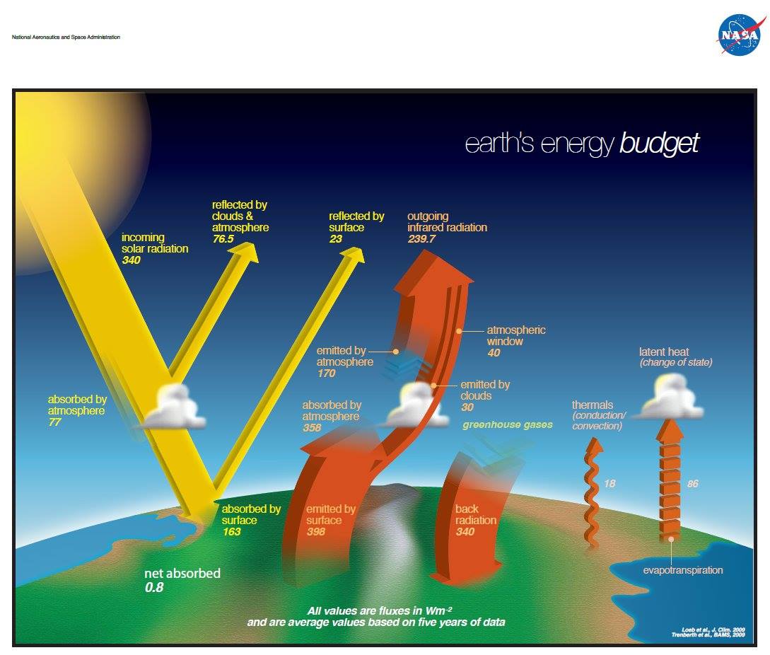 http://science-edu.larc.nasa.gov/energy_budget/ As we said above, the “Emitted by Clouds” label is not given in the original KT97 diagram. Instead, as they say: “The atmospheric emitted radiation is apportioned into two parts to show the LWCF of 30 W/m2”. Here LWCF stands for longwave cloud forcing, which is defined as the difference of the clear-sky and the all-sky outgoing longwave radiation; and also, the difference of the all-sky and clear-sky greenhouse effects, therefore called also the greenhouse effect of clouds. With the data in the KT97 paper, LWCF = 265 – 235 = 155 – 125 = 30 W/m2. |
|||||||||||||||||||||||||||||||||||||||||||||||||||||||||||||||||||||||||||||||||||||||||||||||||||||||||||||||||||||||||||||||||||||||||||||||||||||||||||||||||||||||||||||||||||||||||||||||||||||||||||||||||||||||||||||||||||||||||||||||||||||||
19.§.
But
LWCF, defined as above, is the reduction of outgoing radiation in the
presence of clouds; in itself it is not a contributing component of all-sky outgoing radiation. To attach an arrow for it as a composing element of OLR is not correct. It is not a part of OLR, either this or that way. Maybe this problem was recognized by some authors of the later published energy budget diagrams, because there LWCF is not displayed; see for example the figure of Stevens and Schwartz (2012) from the same Observing and Modeling Earth’s Energy Flows Special Issue of Surveys in Geophysics, altough in the text LWCF (as LW CRE) is given from CERES EBAF as 26.5 W/m2. 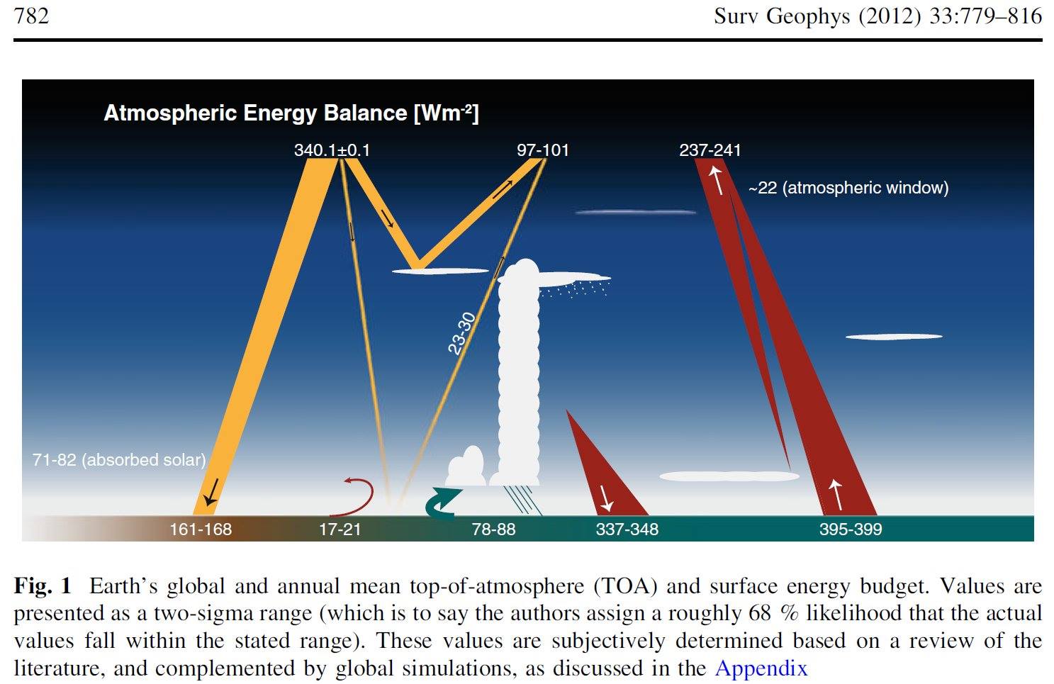 |
|||||||||||||||||||||||||||||||||||||||||||||||||||||||||||||||||||||||||||||||||||||||||||||||||||||||||||||||||||||||||||||||||||||||||||||||||||||||||||||||||||||||||||||||||||||||||||||||||||||||||||||||||||||||||||||||||||||||||||||||||||||||
20.§. The
only exception where the LWCF is still shown is the diagram in
An update on Earth's energy balance in light of the latest global observations G. Stephens, J. Li, M. Wild, C. Clayson, N. Loeb, S. Kato, T. L'Ecuyer, P. Stackhouse, M. Lebsock, T. Andrews (2012) Nature Geoscience 5: 691-696 Its value, according to the latest CERES satellite observations, is updated from 30 W/m2 to 26.6 W/m2. Below we turn back to this diagram in more detail. |
|||||||||||||||||||||||||||||||||||||||||||||||||||||||||||||||||||||||||||||||||||||||||||||||||||||||||||||||||||||||||||||||||||||||||||||||||||||||||||||||||||||||||||||||||||||||||||||||||||||||||||||||||||||||||||||||||||||||||||||||||||||||
21.§. Analysis
of
Stephens et al. (2012) Nature Geoscience An update on Earth's energy balance in light of the latest global observations PART ONE: Data and equations Incoming
solar radiation (ISR) = 340.2±0.1, reflected solar radiation (RSR) =
100.0 ± 2, All-sky
atmospheric window, STI(all), is given as 20 ± 4 W/m2, lower than 22
W/m2 of TF12. LWQ = – (SAA + SH + LH), being equal evidently to
the net LW emission of the column: |
|||||||||||||||||||||||||||||||||||||||||||||||||||||||||||||||||||||||||||||||||||||||||||||||||||||||||||||||||||||||||||||||||||||||||||||||||||||||||||||||||||||||||||||||||||||||||||||||||||||||||||||||||||||||||||||||||||||||||||||||||||||||
|
Stephens
et al. (2012) Nature Geoscience
PART TWO: Relations Note also that with the better window value (22 W/m2), LAA would be 398 – 22 = 376 W/m2, which is the double of –LWQ = 187.9 W/m2: LAA + 2LWQ = 0. This means that the gross longwave absorption of the atmosphere is the double of its longwave cooling. Further, let us realize here that another unexplained relationship can be revealed from the data: DLR – LWQ = 2OLR(all) + 2LWCRE + IMB = 2OLR(clear) + IMB within 0.1 W/m2: 345.6 + 187.9 = 533.5 = 2 × 239.7 + 2 × 26.7 + 0.6 = 2 × 266.4 + 0.6, contrary to the noted ± 9 W/m2 or even ± 12.5 W/m2 uncertainties. What does this equality describe? Total atmospheric LW emission is not a free variable of the IR-absorber composition of the atmosphere but being determined completely by the energy flows at the upper boundary. We were not able to find any reference or expression of this equation, either in the paper or anywhere in the literature. |
|||||||||||||||||||||||||||||||||||||||||||||||||||||||||||||||||||||||||||||||||||||||||||||||||||||||||||||||||||||||||||||||||||||||||||||||||||||||||||||||||||||||||||||||||||||||||||||||||||||||||||||||||||||||||||||||||||||||||||||||||||||||
23.§. Stephens
et al. (2012) Nature Geoscience
PART THREE: Periodicities It
is easy to realize that surface emission, outgoing radiation and
downward atmospheric emission
OLR(all) = 239.7 = 9 LWCE + 0.3 W/m2 OLR(clear) = 266.4 = 10 LWCE + 0.4 W/m2 DLR(clear) = 319 = 12 LWCE – 0.2 W/m2 DLR(all) = 345.6 = 13 LWCE – 0.2 W/m2 LWQ = ULW – OLR – DLR = –187.3 = – 7 LWCE – 1.1 W/m2 G(clear) = ULW – OLR(clear) = 131.6 = 5LWCE – 1.4 W/m2 G(all) = ULW – OLR(all) = 158.3 = 6LWCE – 1.3 W/m2 NSL(all) = ULW – DLR(all) = 52.4 = 2LWCE – 0.8 W/m2 NSL(clear) = ULW – DLR(clear) = 79 = 3LWCE – 0.8 W/m2.
NSL(clear) = 3 G(clear) = 5 G(all) = 6 – LWQ = 7 OLR(all) = 9 OLR(clear) = 10 DLR(clear) = 12 DLR(all) = 13 ULW = 15 units,
|
|||||||||||||||||||||||||||||||||||||||||||||||||||||||||||||||||||||||||||||||||||||||||||||||||||||||||||||||||||||||||||||||||||||||||||||||||||||||||||||||||||||||||||||||||||||||||||||||||||||||||||||||||||||||||||||||||||||||||||||||||||||||
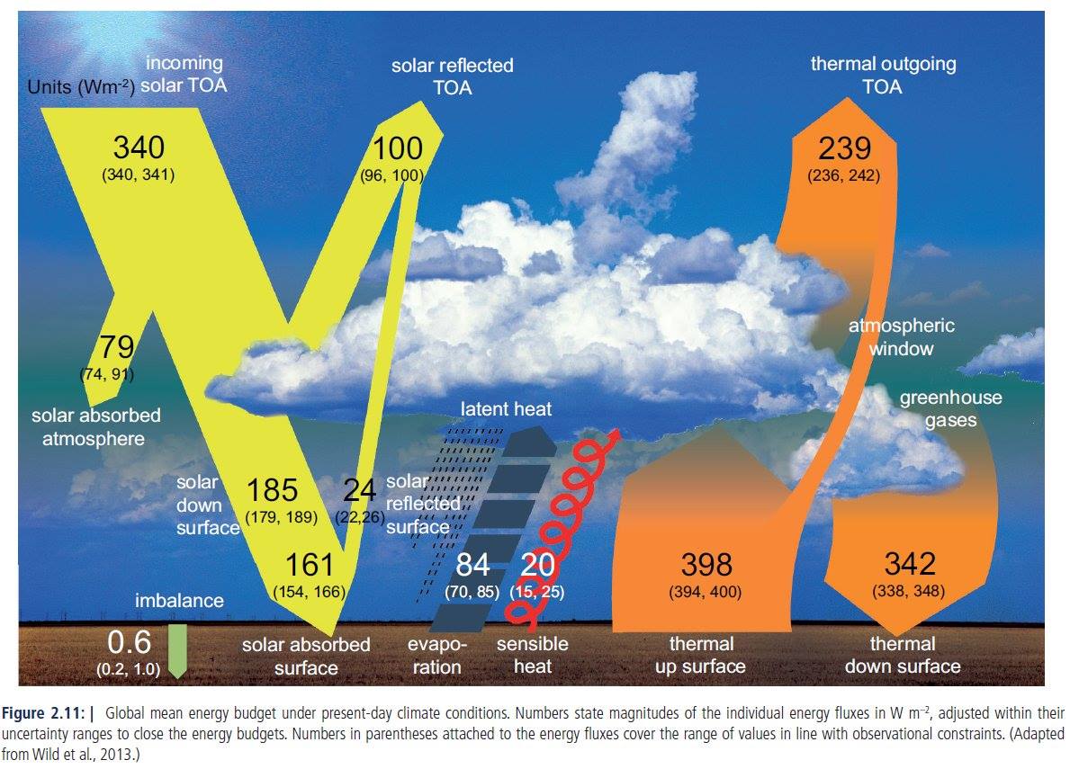
24.§.
IPCC 2013 WGI AR5 Fig
2.11Absorbed solar radiation, ASR = 240 ± 2 W/m2; solar absorbed atmosphere, SAA = 79 ± 5 W/m2; solar absorbed surface, SAS = 161 ± 5 W/m2. Sensible and latent heat, SH + LH = 104 ± 10 W/m2. Greenhouse effect, G = 398 – 239 = 159 ± 3 W/m2; longwave cooling, LWQ = 398 – 239 – 342 = –183 ± 5 W/m2 = – (SAA + SH + LH). No window radiation, no atmospheric LW absorption, no atmospheric upward emission. LWCRE also missing. This diagram is totally inappropriate to make any prediction on the future of the planetary emissivity or the atmospheric opacity.
|
|||||||||||||||||||||||||||||||||||||||||||||||||||||||||||||||||||||||||||||||||||||||||||||||||||||||||||||||||||||||||||||||||||||||||||||||||||||||||||||||||||||||||||||||||||||||||||||||||||||||||||||||||||||||||||||||||||||||||||||||||||||||
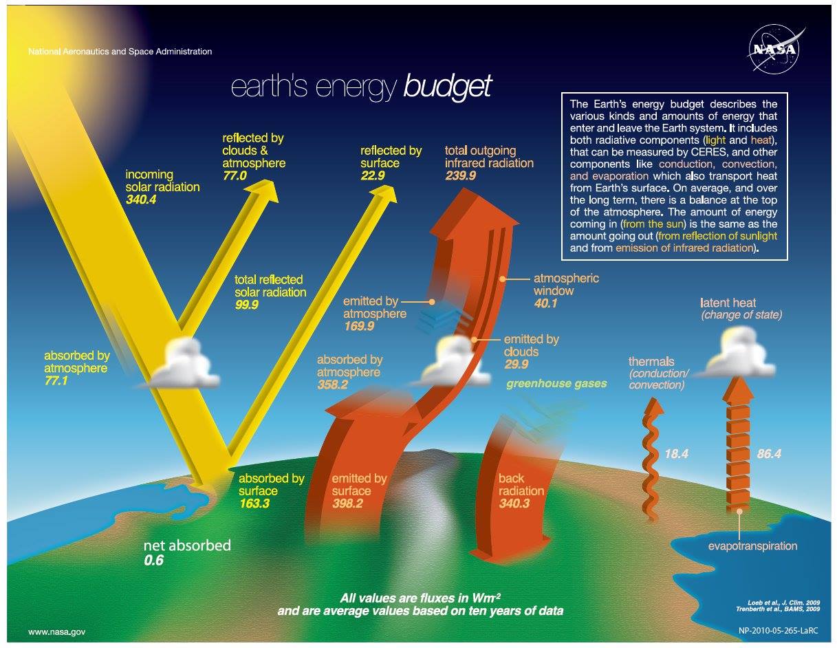
25.§.
NASA
Langley Research Center's Global Energy Budget Poster, June 2014. Some values are evidently outdated: atmospheric window is still from the KT1997 paper, hence atmospheric LW absorption and upward emission are also wrong. No error bounds, problematic decimal numbers, wrong "emitted by clouds". Note that this inaccurate diagram represents Earth's energy budget in Wikipedia.
http://science-edu.larc.nasa.gov/energy_budget/ |
|||||||||||||||||||||||||||||||||||||||||||||||||||||||||||||||||||||||||||||||||||||||||||||||||||||||||||||||||||||||||||||||||||||||||||||||||||||||||||||||||||||||||||||||||||||||||||||||||||||||||||||||||||||||||||||||||||||||||||||||||||||||
|
26.§.
UK
Royal
Society - US National Academy of Sciences 2014:Letter from the American
Association for the Advancement of Science (AAAS) to the Members of
Congress (June 28, 2016)
"reflects the scientific consensus represented by, for example, the U.S. Global Change Research Program, the U.S. National Academies, and Intergovernmental Panel on Climate Change." As we have shown above, the IPCC diagram, as well as their text, is in serious lack of essential climate parameters: neither window radiation, nor atmospheric LW absorption, atmospheric upward emission, clear-sky outgoing radiation or LW cloud effect is quantified. The case is worse with the other two references: Climate Change: Evidence & Causes Their presentation is unsuccessful, unaccectable, oversimplified. The diagram is totally inadequate to explain the greenhouse effect. No solar atmospheric absorption, no sensible and latent heat, no clouds ... and no data. "Some" ?!  * 27.§.
U.S.
Global Change Research ProgramClimate Change Impacts in the United Sates, Appendix 3: Climate Science Supplement. None of the essential parameters are given, the conclusion is unsupported: 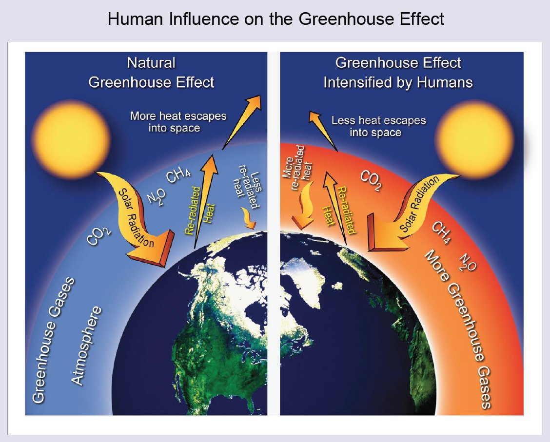 *
28.§. Modified uncertainty ranges (159-165±6, 17-24±7, 80-88±10) make no sense; the statement in the figure legend: "It demonstrates that our scientific understanding of how the greenhouse effect operates is, in fact, accurate" is not supported. |
|||||||||||||||||||||||||||||||||||||||||||||||||||||||||||||||||||||||||||||||||||||||||||||||||||||||||||||||||||||||||||||||||||||||||||||||||||||||||||||||||||||||||||||||||||||||||||||||||||||||||||||||||||||||||||||||||||||||||||||||||||||||
|
29.§.
A slightly modified
version of the IPCC 2013 diagram is given in:Wild et al. (2015) The energy balance over land and oceans Clim Dyn 44: 3393–3429
|
|||||||||||||||||||||||||||||||||||||||||||||||||||||||||||||||||||||||||||||||||||||||||||||||||||||||||||||||||||||||||||||||||||||||||||||||||||||||||||||||||||||||||||||||||||||||||||||||||||||||||||||||||||||||||||||||||||||||||||||||||||||||
|
30.§.
L'Ecuyer
et al. (2015)The Observed State of the Energy Budget in the Early Twenty-First Century Journal of Climate 28: 8319 – 834 An important effort is presented by L'Ecuyer et al. (2015): an 'objectively balanced observation-based reconstruction' of the energy budget is promised, where relevant energy and water cycle constraints were applied on the satellite observations. They say that in the absence of these constraints, the observed energy budget looks like this (see below their Fig. 1), while the constrained structure is given in their Fig. 4: 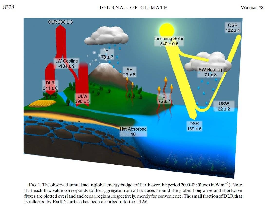  The data are presented in a table as well: 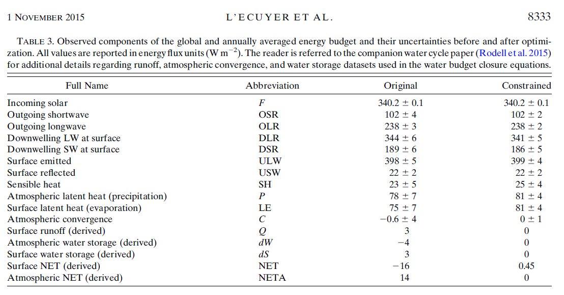 |
|||||||||||||||||||||||||||||||||||||||||||||||||||||||||||||||||||||||||||||||||||||||||||||||||||||||||||||||||||||||||||||||||||||||||||||||||||||||||||||||||||||||||||||||||||||||||||||||||||||||||||||||||||||||||||||||||||||||||||||||||||||||
|
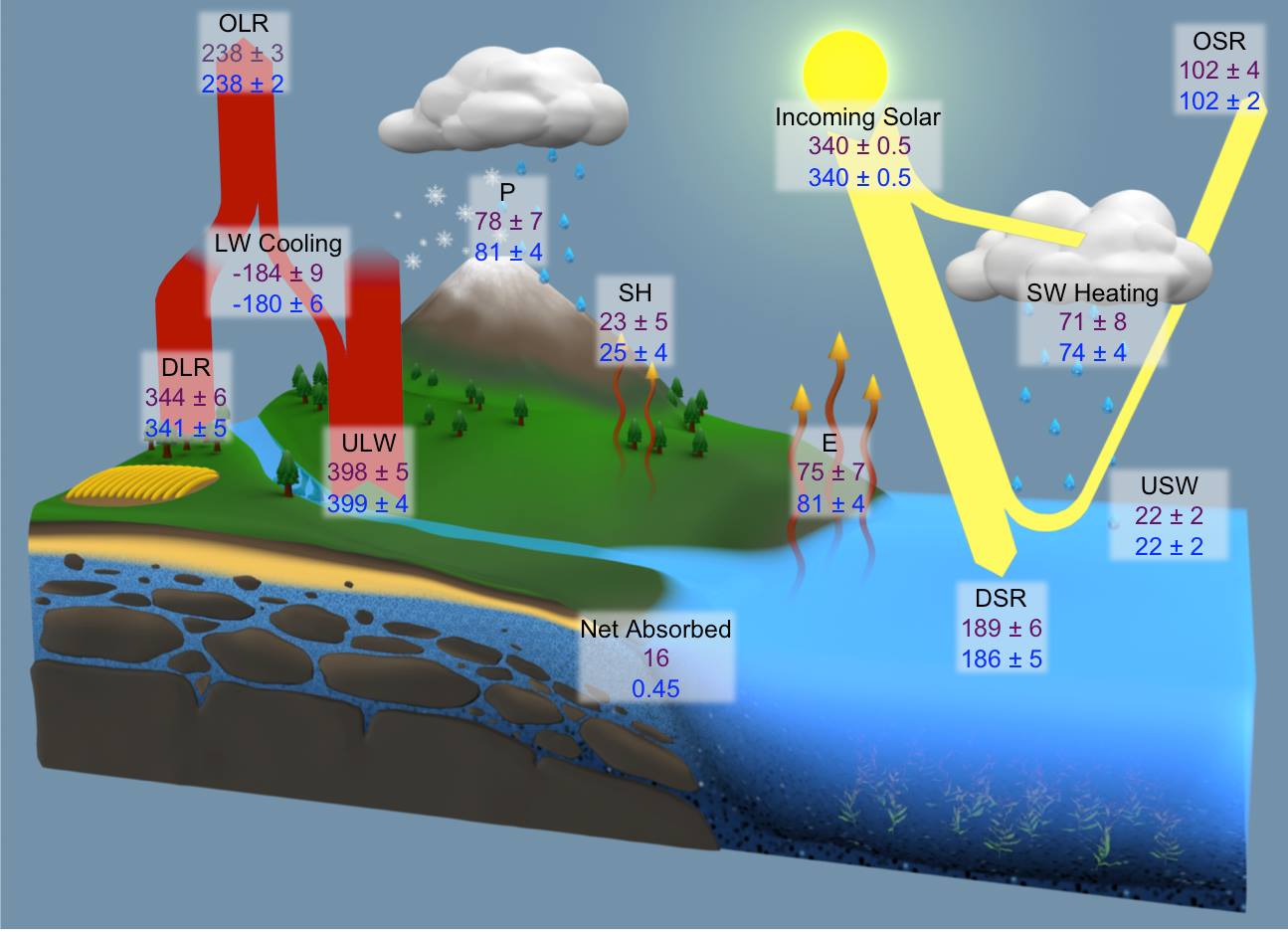
31.§. Stephens
and L'Ecuyer (2015): The
Earth's energy balance
Atmospheric Research 166: 195–203 But something must have gone wrong with the 'objectively balanced' first optimization, since an immediate update became necessary to the L'Ecuyer et al. (2015) paper (available online on the same week): Stephens and L'Ecuyer (2015) applied an (even-more objectively balanced) 'second optimization', where two fundamental energy budget parameters, DLR and LW Cooling, were taken back to their original, observed, unconstrained value. First diagram below: L'Ecuyer et al. with observed and the constrained data. Second diagram: Stephens and L'Ecuyer, with the first-optimized, and the second-optimized data. LW Cooling = ULW – OLR – DLR = – (SH + E + SW Heating).
This is the latest detailed study we were able to find in the literature on Earth's global energy budget. As we noted in the Introduction, its substantial feature is the unequivocal E(SRF) — E(TOA) connection. E(SRF) = DSR – USW + DLR = ULW + SH + E = 185 – 22 + 344 = 399 + 26 + 82 = 507 W/m2. Imbalance (Net Absorbed) = 0.45 W/m2 OLR = 240 W/m2. LWCRE from the Stephens-Li-Wild-Clayon-Loeb-Kato-L'Ecuyer et al. Nature Geosci (2012) paper: LWCRE = 26.6 W/m2. We can find here a nowhere-mentioned, never-declared, not-explained relationship: E(SRF) = 2OLR + LWCRE + IMB = 507 W/m2 = 2 × 240 + 26.6 + 0.4 W/m2. Let us declare: Our fundamental, 'effectively closed' greenhouse relationship, which is based on our 'leaky glass-shell' concept as detailed in the Introduction, is fulfilled exactly in the most recently created energy budget diagram. The principal relationship is that the energy flows at the surface are equal to the total (incoming plus outgoing) energy flows at TOA plus the greenhouse effect of clouds. |
|||||||||||||||||||||||||||||||||||||||||||||||||||||||||||||||||||||||||||||||||||||||||||||||||||||||||||||||||||||||||||||||||||||||||||||||||||||||||||||||||||||||||||||||||||||||||||||||||||||||||||||||||||||||||||||||||||||||||||||||||||||||
32.§.
Earth's energy budget, based on IPCC
(2013), is represented this
way in P. Read et al. (2015):Two
other diagrams, published later, but with earlier data:
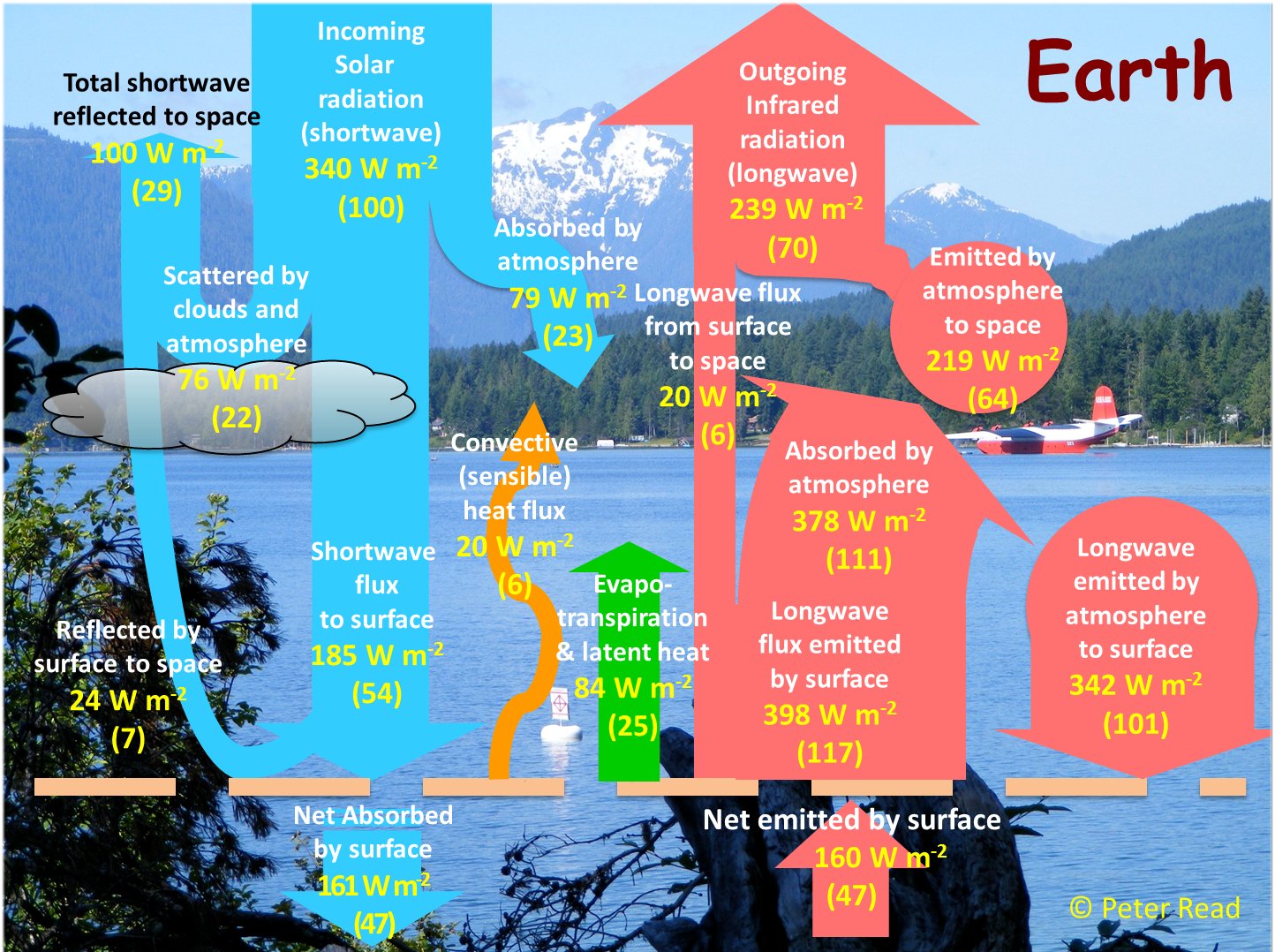 Global
energy budgets and 'Trenberth diagrams' for the climates of
terrestrial and gas giant planets
QJRMS 142: 703-720. 33.§.
Loeb (2015) in a presentation repeated his
own 2014 diagram, with the following estimate for the Earth's energy budget: OLR = 240 ± 2 W/m2 LWQ ( LW Cooling) = – 187 ± 8 W/m2 SAA (solar absorbed by atmosphere) = 78 ± 5 W/m2 SH (sensible heat) = 24 ± 7 W/m2 LH (latent heat) = 78 ± 6 W/m2 Clear-sky and cloudy reflections and emissions are noted, but not quantified. 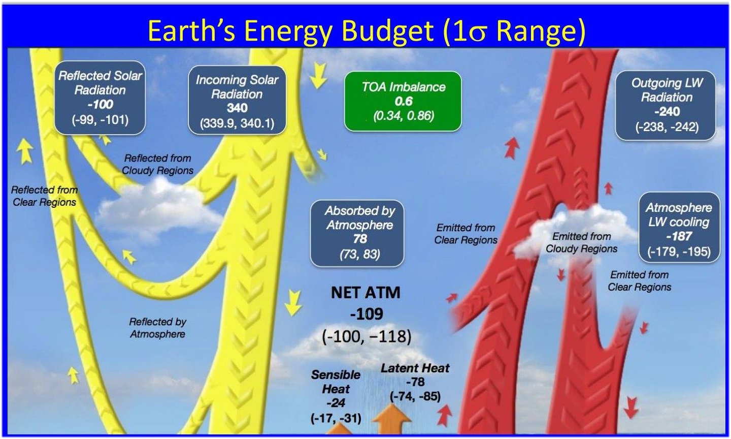 Loeb N (2015) Radiation at the top of the atmosphere. Presentation at the Workshop on energy flow through the climate system. Met Office UK, Exeter, 30 Sept 2015. BREAKING NEWS NASA LaRC website http://science-edu.larc.nasa.gov/energy_budget/ added New 2016 Revision 7 Earth's Radiation Budget Litograph:  NASA Earth Radiation Budget Diagram created 13 June 2016 [pdf, 21 MB] atmosheric window: 11.8 % of incoming sunlight = 40 W/m2 emitted by clouds: 8.8 % = 30 W/m2. The same old, inaccurate, outdated numbers as in the 2014 version. * The atmospheric energy balance equation was also 'lost' in the maintime: The 2014 version:  The 2016 version:  |
|||||||||||||||||||||||||||||||||||||||||||||||||||||||||||||||||||||||||||||||||||||||||||||||||||||||||||||||||||||||||||||||||||||||||||||||||||||||||||||||||||||||||||||||||||||||||||||||||||||||||||||||||||||||||||||||||||||||||||||||||||||||
|
34.§.
Cloud
Area FractionKiehl and Trenberth (1997) mention a total cloud area fraction of beta = 62%, but when computing the all-sky atmospheric window from their clear-sky value as 40 W/m2 = (1 – 0.6) × 99 W/m2, they calculate with a cloud area fraction of 60%. CERES SYN1deg product version Ed3A presents data from March 2000 to April 2016. It starts with a mean value of about 62%, then shows a slight decrease to an average of 0.605 for the last seven years. *** Kiehl and Trenberth, with beta = 0.62, had an albedo of 0.31. ISCCP, with beta = 0.67, had the albedo at 0.33 (Rossow and Zhang 1995). Beta = 0.6 is consistent with a planetary albedo of 0.293. *** Measurement descriptions mention uncertainties coming from the handling of cloud overlap: the actually observed multi-layer cloud area fraction is corrected to get the single-layer fraction. *** There are also concerns with objects like haze, fog and very thin clouds; these might have more than zero infrared optical depth. *** It seems well-founded to regard the effective IR-opaque single-layer geometric cloud area fraction β0 = 0.6. 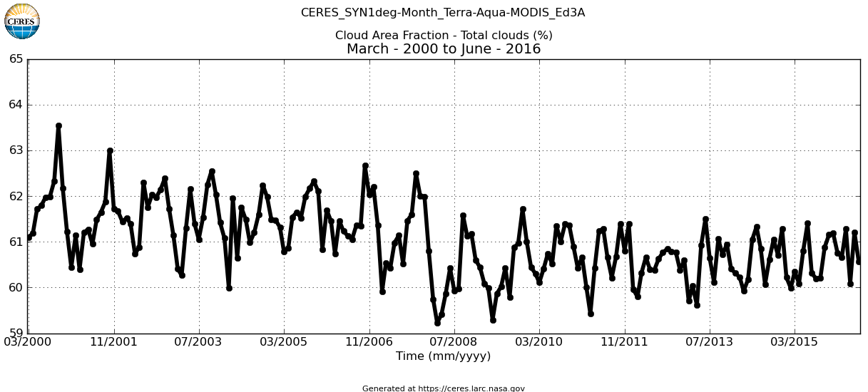 |
|||||||||||||||||||||||||||||||||||||||||||||||||||||||||||||||||||||||||||||||||||||||||||||||||||||||||||||||||||||||||||||||||||||||||||||||||||||||||||||||||||||||||||||||||||||||||||||||||||||||||||||||||||||||||||||||||||||||||||||||||||||||
35.§.
Results We present here all F fluxes in the Earth's energy flow system (solar atmospheric and surface absorptions, longwave absorptions and emissions, non-radiative fluxes as sensible and latent heat, observable and only-computable radiations as window radiation or upward atmospheric emission) as F = F0 + Delta F, where Delta F is a small fluctuation (due to observation errors or systematic deviations, typically within the ±2 W/m2 range, which is less than ±1 sigma), F0 = N × UNIT, N is an integer, and the unit is UNIT(all) = LWCRE = 26.6 W/m2 for all-sky, UNIT(cloudy) = LWCRE / beta = 44.33 W/m2 for cloudy sky (beta = cloud area fraction) and UNIT(clear) = STI(clear) = 66.5 W/m2 for clear-sky fluxes. We will refer to the F0 values as 'grid' positions. 36.§.
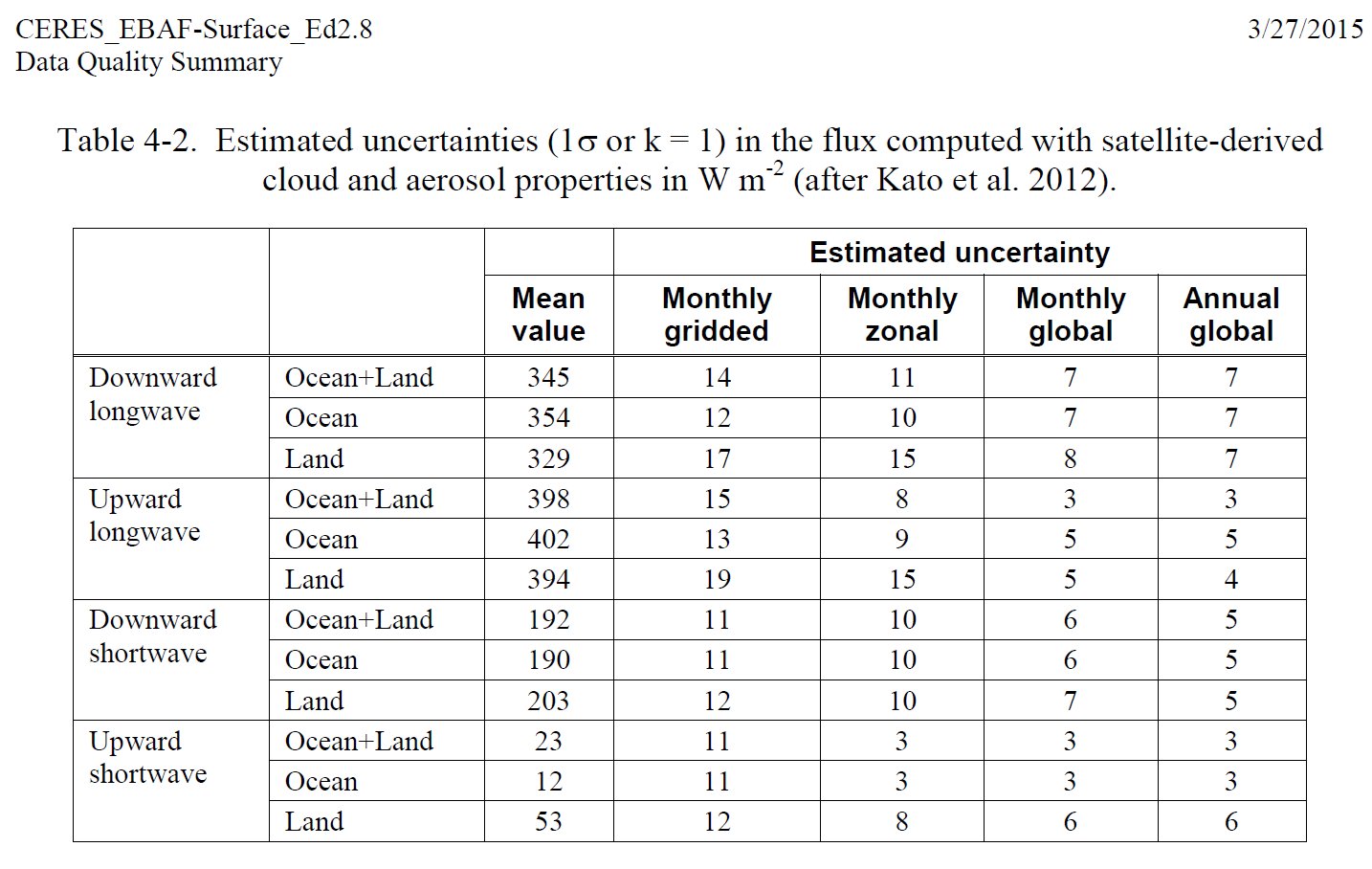
Surveys in Geophysicshad a Special Issue on Observing and Modeling Earth's Energy Flows in 2012. We refer to three of its papers. Kato et al. (2012) in their 'Uncertainty estimate of Surface Irradiances', give the following data: DLR = 345 ± 7 W/m2 ULW = 398 ± 3 W/m2. Trenberth and Fasullo (2012) in their diagram have OLR = 238.5 W/m2. Stevens and Schwartz (2012), based on CERES EBAF, gave LWCRE = OLR(clear) – OLR(all) = 26.5 W/m2. Now it is easy to realize that DLR = 13 LWCRE + 0.5 W/m2 ULW = 15 LWCRE + 0.5 W/m2 OLR = 9 LWCRE precisely. The formula of LWQ = ULW – OLR – DLR expresses LW Cooling of the atmosphere (the LW energy entering into it from below less that leaving it above and below) (see e.g. Stephens et al. 1994: Observations of the Earth's radiation budget; Eq. 9) its value is then LWQ = 398 – 345 – 238.5 = –185.5 W/m2 = – 7 LWCRE exactly. This longwave energy loss of the atmosphere is being balanced by the non-LW energy incomes of the atmosphere: LWQ = – (SAA + SH + LH), where SAA is solar absorbed by atomsphere; SH and LH are sensible and latent heating. Stevens and Schwartz (2012, Table 1) give the sum of surface non-radiative fluxes as SH + LH = 106 W/m2. (Later, L'Ecuyer et al. 2015, based on their detailed global energy and hydrological cycle assessment, repeat this value.) Now it can be seen that SH + LH = 106 = 4 × 26.5 W/m2 = 4 LWCRE exactly. This leaves for SAA = 3 LWCRE = 79.5 W/m2 precisely. With these values, the surface energy balance can be written as E(SRF) = solar absorbed surface + downward longwave radiation = radiative and non-radiative cooling (+ IMB) = 162 + 342 = 398 + 106 = 504 W/m2. It can be realized immediately that it equals to 2OLR + LWCRE: E(ESRF) = 504 W/m2 = 2 × 239 W/m2 + 26 W/m2 with an accurcy of 0.5 W/m2, contrary to the noted much higher 1-sigma uncertainty ranges. If the equality E(SRF) = 2OLR + LWCRE proves to be valid, it might modify our concept about the work of the climate system, as it suggests that the energy at the surface is not a free variable of the atmospheric downward radiation, but being pre-determined by the energy flows at TOA. It can be written also, within some imbalance as: E(SRF) = OLR(all) + OLR(clear) or E(SRF) = ASR + OLR(clear) or E(SRF) = 2ASR + LWCRE. * Surveys in Geophysics released a Special Issue on the Earth's hydrological cycle in 2014; it made possible to refine the value of the latent heat, as it is given there by Bengtsson (2014) as LH = 80 W/m2. This value can be written as LH = 3 LWCRE + 0.5 W/m2, therefore SH = 26.5 W/m2 = 1 LWCRE. which are now another members in the arithmetic sequence of fluxes with a common difference of LWCRE. The surface energy is then becomes the 19th member of the progression: E(SRF) = 19 LWCRE 504 W/m2 = 19 × 26.5 ( + 0.5) W/m2. *** To check the data: Stevens and Schwartz (2012) Surv Geophys, Table 1: Observing and Modeling Earth’s Energy Flows 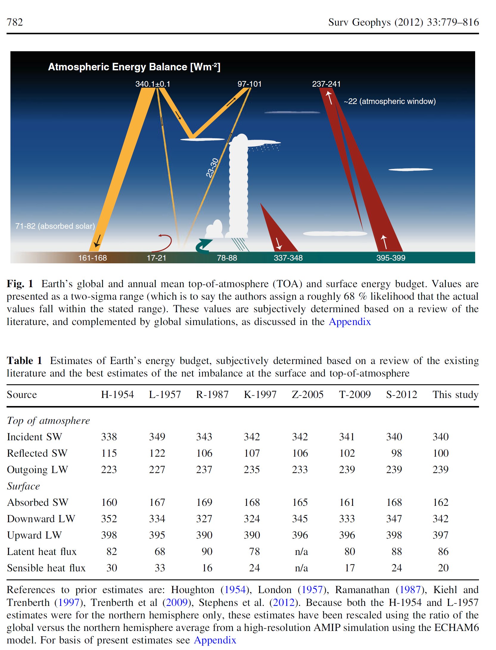 (From Bjorn Stevens • Stephen E. Schwartz Surv Geophys (2012) 33:779–816 DOI 10.1007/s10712-012-9184-0) *** 37.§.
The found pattern in the
Stephens et al. (2012) dataAs noted earlier, the structure can be recognized in the observed data given in the updated energy balance diagram of Stephens et al. (2012) Nature Geoscience. Here we complete this 'periodic table' with the best solar atmospheric absoprtion value from the most recent detailed land-ocean assessment of Wild et al. (2015): SAA = 80 W/m2, and with the updated data given by the simultaneous global energy and water cycle assesment of L'Ecuyer et al. (2015) and Stephens and L'Ecuyer (2015). Sensible heat, SH = 25 W/m2, Latent heat, LH = 81 W/m2, ULW = 399 W/m2. Now we have: F = F0 + Delta
all within a largest difference of 1.6 W/m2, The attached uncertainties (± 1-sigma range) are much larger, typically 4 W/m2 or more. We
are not aware of any mention or reflection to these characteristics of
the energy budget by any of the authors of the Surveys in Geophyscis
Special Issue (2012) or the Stephens et al. Nature Geosci (2012) paper, * E(SRF) = ULW + SH + LH = OLR(all) + OLR(clear) = 2OLR(all) + LWCE. It can also be written, within an imbalance, as
E(SRF) = 2ASR + LWCRE or E(SRF) = ASR + OLR(clear) . *** The atmospheric version of this balance equation can be recognized numerically in the referredStephens et al. (2012) diagram. This equality does not follow from any known balance requirement, and is not mentioned either in the paper or anywhere in the literature; our additions are in green; the proper position of 'window' is also indicated: 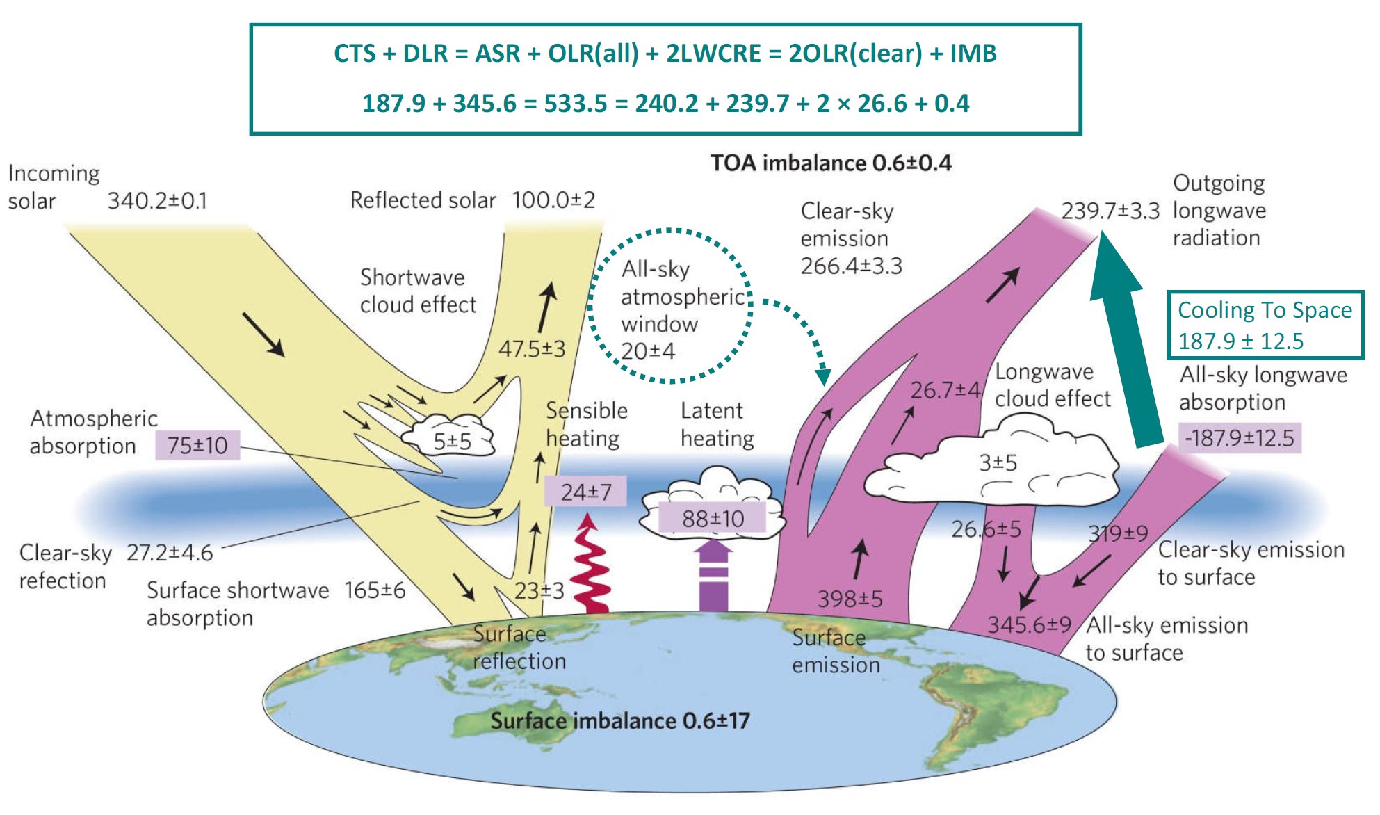 * It can be found, with their own data, in the NASA Langley (2014) poster as well (our addition: yellow and red arrows and white textboxes). 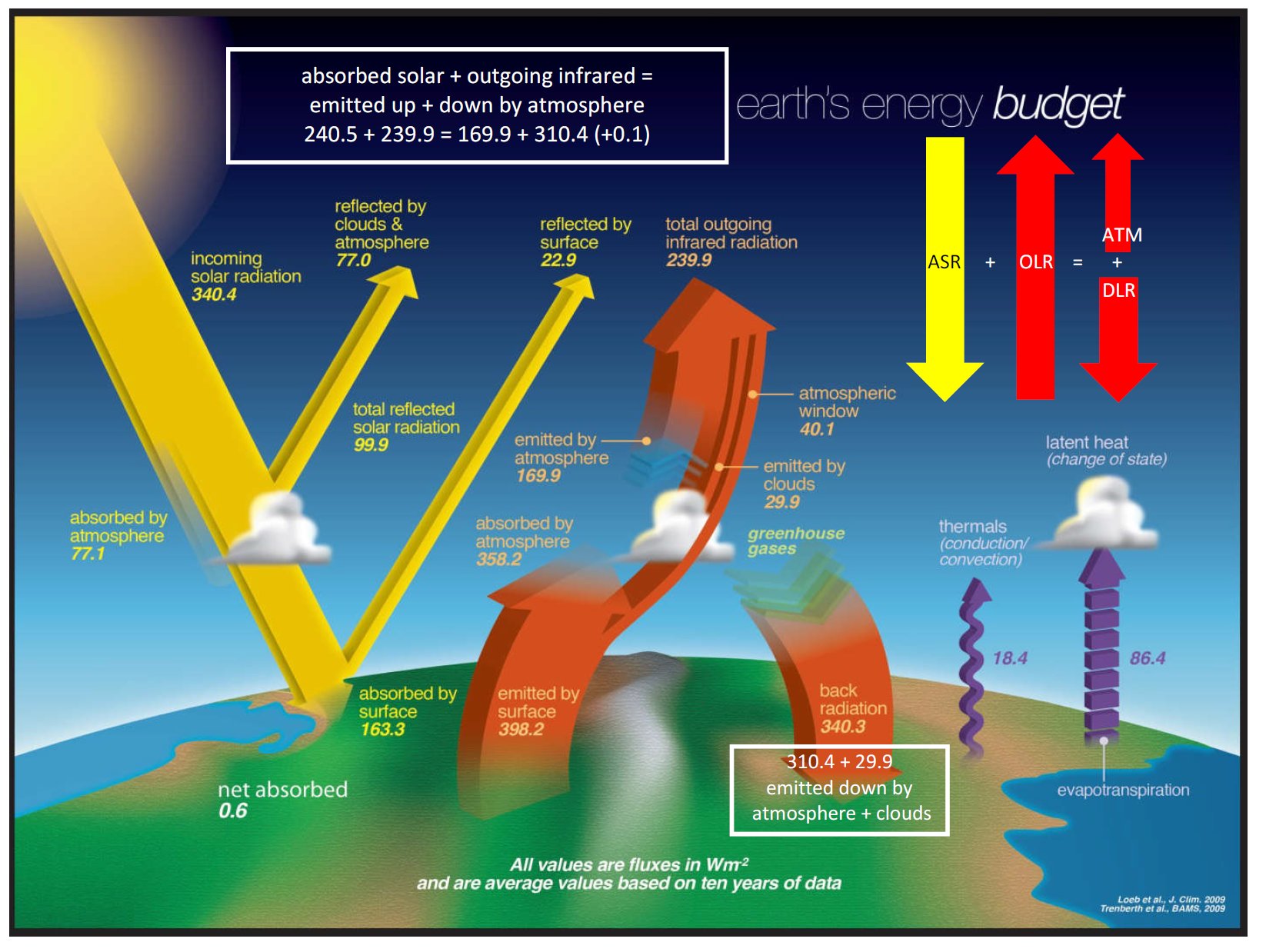 *** We have to emphasize that this relationship: 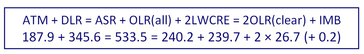  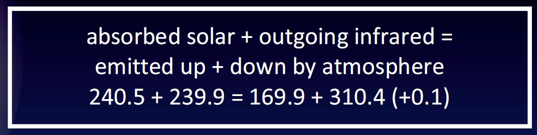 (the strict equality of the total [upward plus downward] atmospheric emissions to the total [absorbed plus emitted] energy flows at TOA, with or without the cloud effect) is valid in two different, but coherent and self-consistent representations. *** This is evidently not the case, for example, in the CO2-atmosphere of the Mars: Read
et al. (2015): Global
energy budgets and 'Trenberth diagrams' for the climates of
terrestrial and gas giant planets. QJRMS
142: 703-720.
ASR = OLR = 110 W/m2, SAA = 14 W/m2, SAS = 96 W/m2, ULW = 123 W/m2, DLR = 27 W/m2, LAA = 33 W/m2, STI = 90 W/m2, CTS = 20 W/m2, G = 13 W/m2. E(SRF, Mars, clear) = SAS + DLR = 96 + 27 = ULW = 123 W/m2 E(ATM, Mars, clear) = SAA + LAA = 14 + 33 = CTS + DLR = 20 + 27 = 47 W/m2 ASR + OLR = 220 W/m2. Mars: ASR + OLR >> CTS + DLR and E(SRF, Mars, clear) << ASR + OLR. * That is, ASR + OLR = CTS + DLR and E(SRF, clear) = 2OLR(clear) are NOT general planetary rules. They are Earth-specific relationships. * On Earth, the surface and atmospheric energy budgets are maximized, and limited (constrained) to (predetermined by) the available energy at TOA. ***
*** But how? More CO2 won't absorb more? Yes, they probably try to absorb more, initially and instantaneously perhaps successfully, but then the limit of the anual global mean blocks the process and regulates back to where it was. Exchange of CO2 and H2O molecules between the atmosphere and the ocean surface, and the created vertical and regional temperature configuration maintain the prescribed energetic construction. *** Before presenting our flux aritmetic progression tables, to make it easy to compare them to the observed data, we show here another data tables from open access publications: Wild et al. (2015) Clim Dyn, Table 3: (The energy balance over land and oceans: an assessment based on direct observations and CMIP5 climate models Martin Wild · Doris Folini · Maria Z. Hakuba · Christoph Schär · Sonia I. Seneviratne · Seiji Kato · David Rutan · Christof Ammann · Eric F. Wood · Gert König‑Langlo DOI 10.1007/s00382-014-2430-z)  * Loeb et al. (2015) Clim Dyn Table 2: Observational constraints on atmospheric and oceanic cross‑equatorial heat transports: revisiting the precipitation asymmetry problem in climate models Norman G. Loeb · Hailan Wang · Anning Cheng · Seiji Kato · John T. Fasullo · Kuan‑Man Xu · Richard P. Allan DOI 10.1007/s00382-015-2766-z 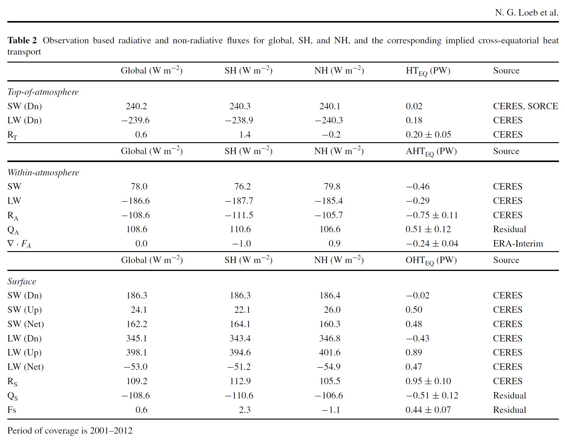 Sigma is taken from Stephens and L'Ecuyer (2015) and from Loeb (2015) Delta is taken from two different studies. STI(all) is computed from STI(clear) = 66.5 W/m2 and β = 0.6. LWCRE = 26.6 W/m2 defined from OLR(clear)/10. 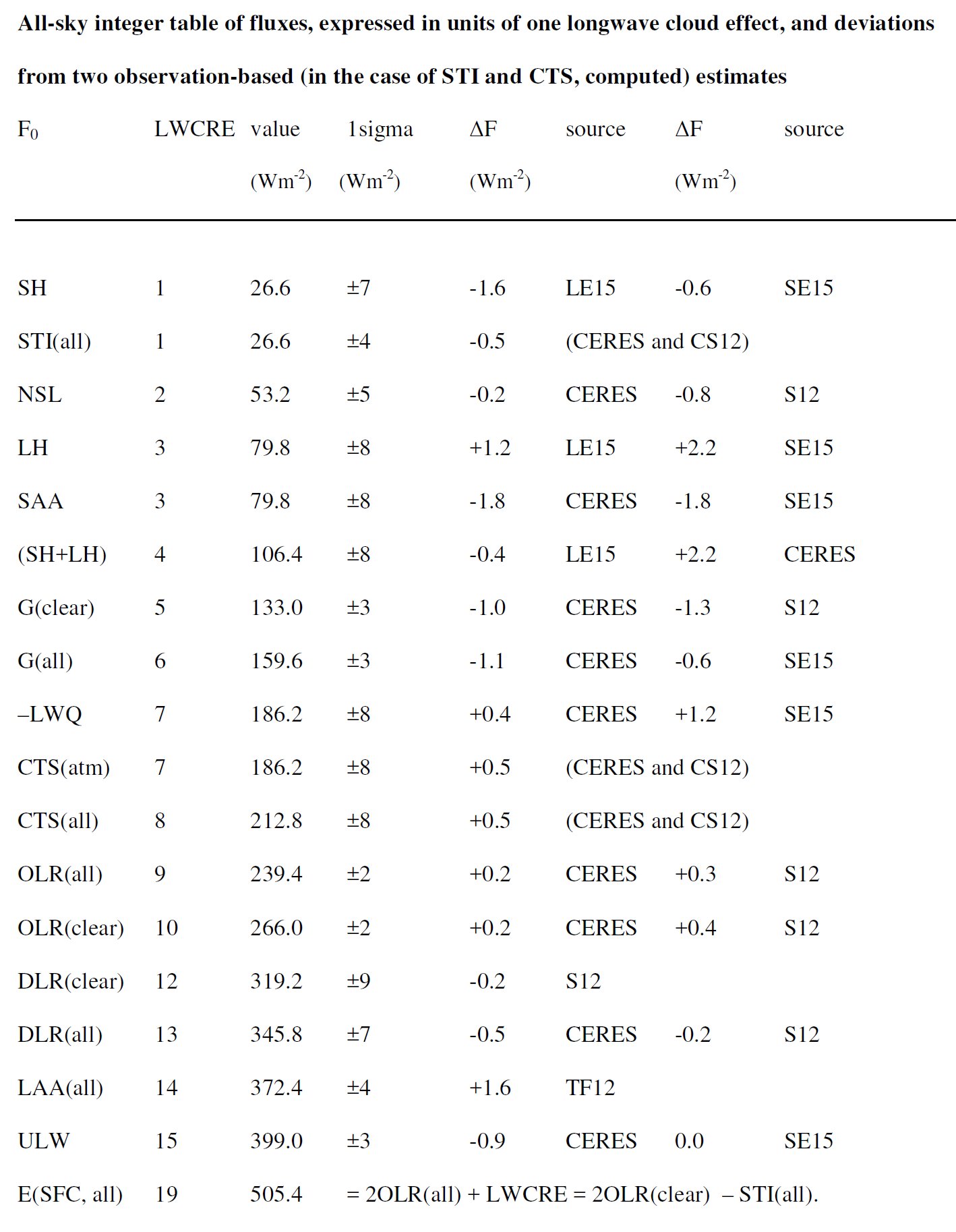 Line 19 says that the energy flows at the surface are predetermined by the energy flows at TOA. If these observed data are correct, it can be seen that the energy flows at the surtface: incoming = solar absorbed surface, SAS + downward longwave radiation, DLR and emitted = upward longwave radiation, ULW plus sensible + latent heat release, SH + LH are completely constrained to the energy flows at TOA, and equal to 2OLR(all) plus one LW cloud effect, within an imbalance less than 1 W/m2: E(SRF) = SAS + DLR = ULW + SH + LH = 2OLR(all) + LWCE = 2OLR(clear) – STI(all). 506.2 = 160.4 + 345.8 = 399.0 + 26.6 + 79.8 ( + 0.8) = 2 × 239.4 + 26.6 (+ 0.8) = 2 × 266.0 – 26.6 (+ 0.8). |
|||||||||||||||||||||||||||||||||||||||||||||||||||||||||||||||||||||||||||||||||||||||||||||||||||||||||||||||||||||||||||||||||||||||||||||||||||||||||||||||||||||||||||||||||||||||||||||||||||||||||||||||||||||||||||||||||||||||||||||||||||||||
39.§.
Flux
progression table, clear skyBesides the all-sky structure, where the unit flux was LWCE = 26.6 W/m2, there is also a clear-sky pattern, with the unit of STI(clear) = 66.5 W/m2. Further, the amount of energy flows at the surface can be calculated as follows. Absorbed solar radiation in the climate system under cloud-free skies, from CERES-EBAF, is ASR(clear) = 287 W/m2; higher than the clear-sky OLR of 266 W/m2. The clear and the cloudy subsets of the atmosphere in themselves are not in equilibrium; energy exchange must appear between the two: the 21 W/m2 clear-sky surplus in the all-sky global average means (1 – β) × 21 = 8.4 W/m2, therefore 8.4 / β = 14 W/m2 must appear in the cloudy part.. Using ASR(clear) = 287 W/m2, the best estimate for the cloud-free surface atmospheric absorption is SAS(clear) = 213 W/m2, which leaves for solar absorption by the atmosphere SAA(clear) = 74 W/m2. Together with DLR(clear) = 319 W/m2 (Stephens et al. 2012) we have the surface energy income under clear-sky as E(SRF, clear) = SAS(clear) + DLR(clear) = 532 W/m2. It can be immediately recognized that this equals to 2OLR(clear): E(SRF, clear) = SAS(clear) + DLR(clear) = 2 OLR(clear). (See more below in the Discussion of the cooling-to-space approximation in 56.§ and the Clear-sky pattern in 63.§) In the all-sky case, the connection between the atmospheric LW absorption and downward LW emission is LAA(all) – DLR(all) = 26.6 W/m2 = 1 LWCRE. |
|||||||||||||||||||||||||||||||||||||||||||||||||||||||||||||||||||||||||||||||||||||||||||||||||||||||||||||||||||||||||||||||||||||||||||||||||||||||||||||||||||||||||||||||||||||||||||||||||||||||||||||||||||||||||||||||||||||||||||||||||||||||
|
40.§.
Flux progression table, cloudy
skyUnit: LWCRE / β Cloud area fraction enables us to establish the cloudy flux structure . If the cloud cover is opaque in the infrared, the surface transmitted irradiance is zero: STI(cloudy)=0. Therefore CTS(all, cloudy) = OLR(cloudy) – STI(cloudy) = OLR(cloudy) and CTS(atm, cloudy) = OLR(cloudy) – LWCRE/ β, with OLR(cloudy) = OLR(clear) – LWCRE/ β. With a value of β0 = 0.6, we have OLR(clear) – OLR(cloudy) = LWCRE / β = 26.6 / 0.6 = 44.33 W/m2. In this unit, the cloudy periodic table is the following, see Table 4: 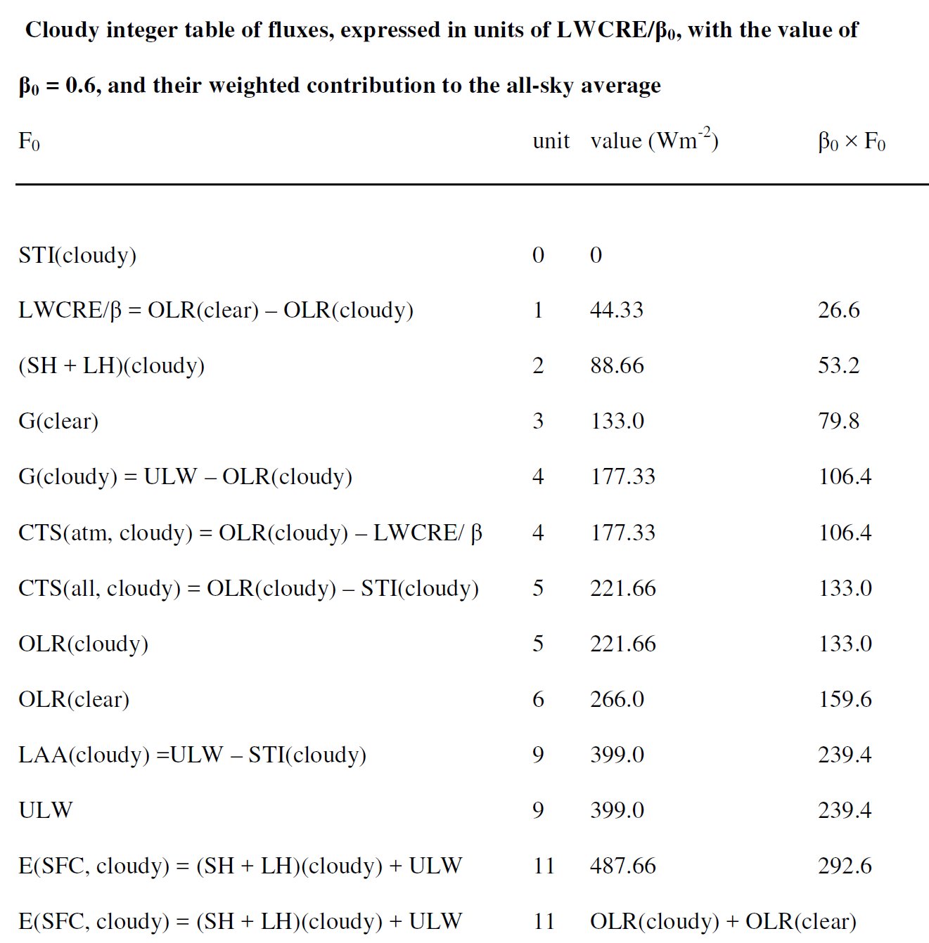 Downward LW radiation under cloudy skies, from the definition of DLR(all) = β × DLR(cloudy) + (1 – β) × DLR(clear) is DLR(all) = 363.53 W/m2. The cloudy-sky difference of LW absorption and downward emission is then LAA(cloudy) – DLR(cloudy) = 35.47 W/m2. The global contribution of the clear-sky difference of 13.3 W/m2 is 0.4 × 13.3 = 5.32 W/m2; The global contribution of the cloudy-sky difference of 35.47 W/m2 is 0.6 × 35.47 = 21.28 W/m2, hence the global average all-sky difference of these two fluxes is 5.32 + 21.28 = 26.6 W/m2 = LWCRE. *** Clear and cloudy fluxes can be compared to, for example: 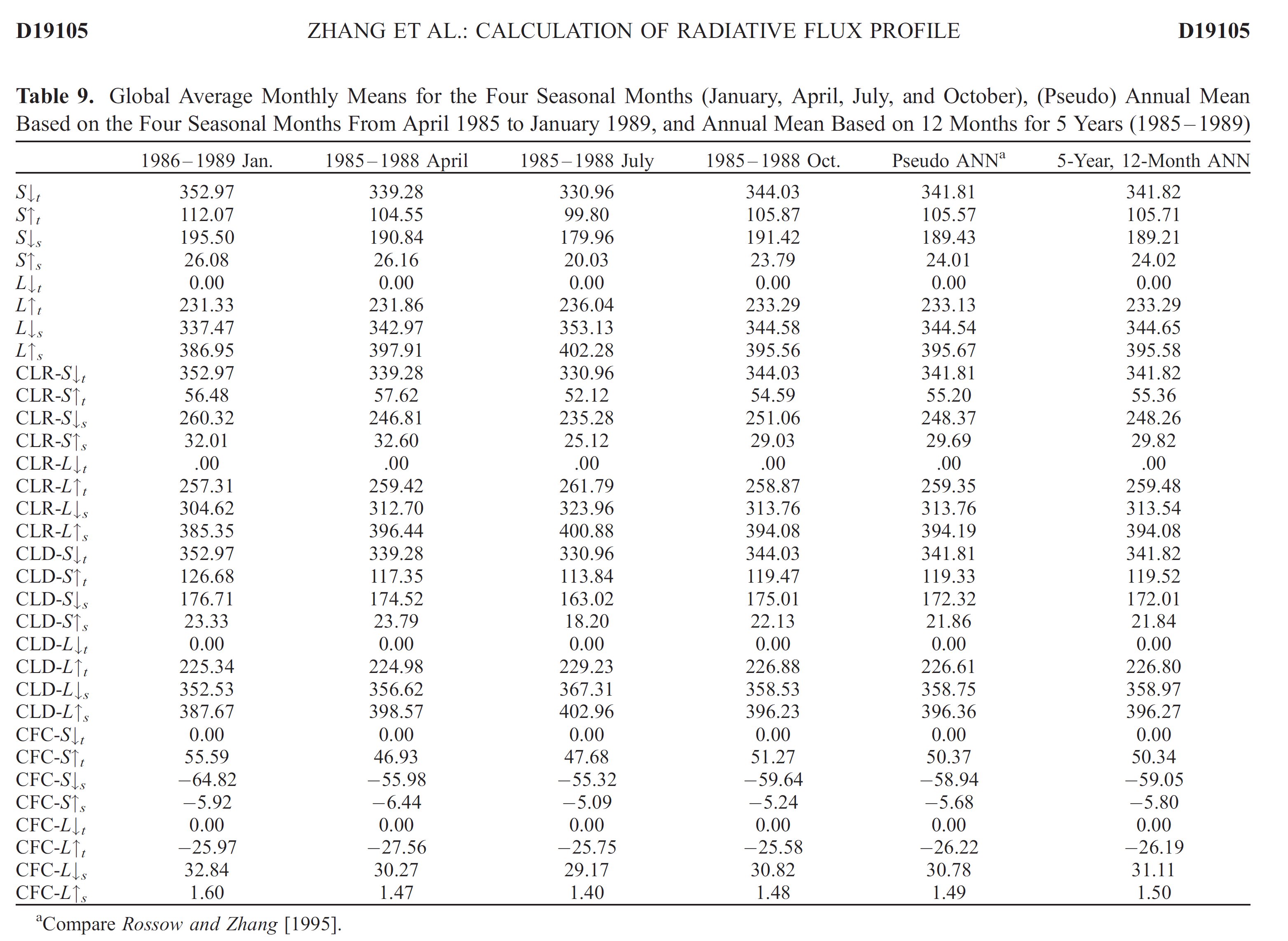 Zhang, Rossow, Lacis, Oinas, Mischenko (2004): Calculation of radiative fluxes from the surface to top of atmosphere based on ISCCP and other global data sets: Refinements of the radiative transfer model and the input data. JOURNAL OF GEOPHYSICAL RESEARCH, VOL. 109, D19105, doi:10.1029/2003JD004457, 2004 * The differences are smaller than the CERES EBAF TOA flux adjustments: 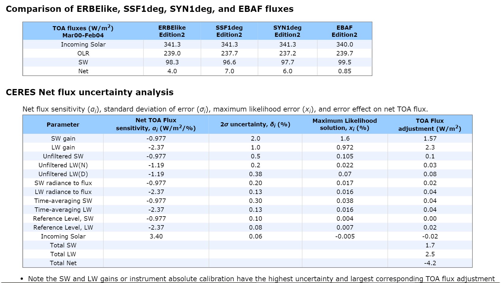 http://ceres.larc.nasa.gov/science_information.php?page=EBAFbalance Let us compare the Earth cloudy flux relationships to the Martian dusty case: 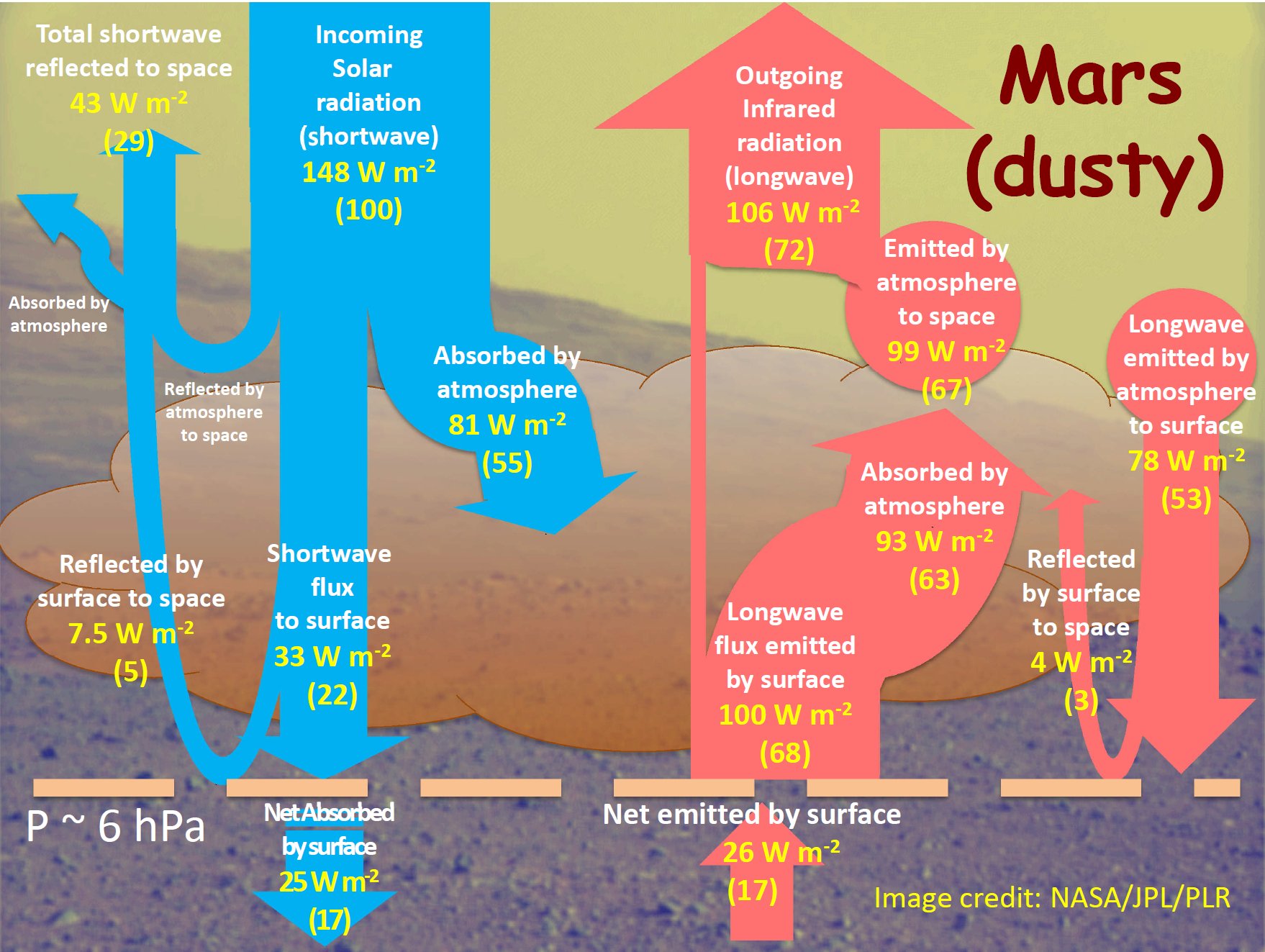 Read
et al. (2015): Global
energy budgets and 'Trenberth diagrams' for the climates of
terrestrial and gas giant planets. QJRMS
142: 703-720.
ASR = OLR = 106 W/m2, SAA = 81 W/m2, SAS = 25 W/m2, LAA = 93 W/m2, STI = 7 W/m2 ULW = 100 W/m2, CTS = 99 W/m2, DLR = 75 W/m2, G(dusty) = 6 W/m2 E(SRF, Mars, dusty) = 25 + 75 = 100 W/m2 E(ATM, Mars, dusty) = 81 + 93 = 99 + 75 = 174 W/m2 E(SRF, Mars, dusty) << OLR(dusty) + OLR(clear) E(ATM, Mars, dusty) < OLR(dusty) + OLR(clear) * |
|||||||||||||||||||||||||||||||||||||||||||||||||||||||||||||||||||||||||||||||||||||||||||||||||||||||||||||||||||||||||||||||||||||||||||||||||||||||||||||||||||||||||||||||||||||||||||||||||||||||||||||||||||||||||||||||||||||||||||||||||||||||
Our poster Global enegy budget, flux progression tables and the greenhouse effect of clouds 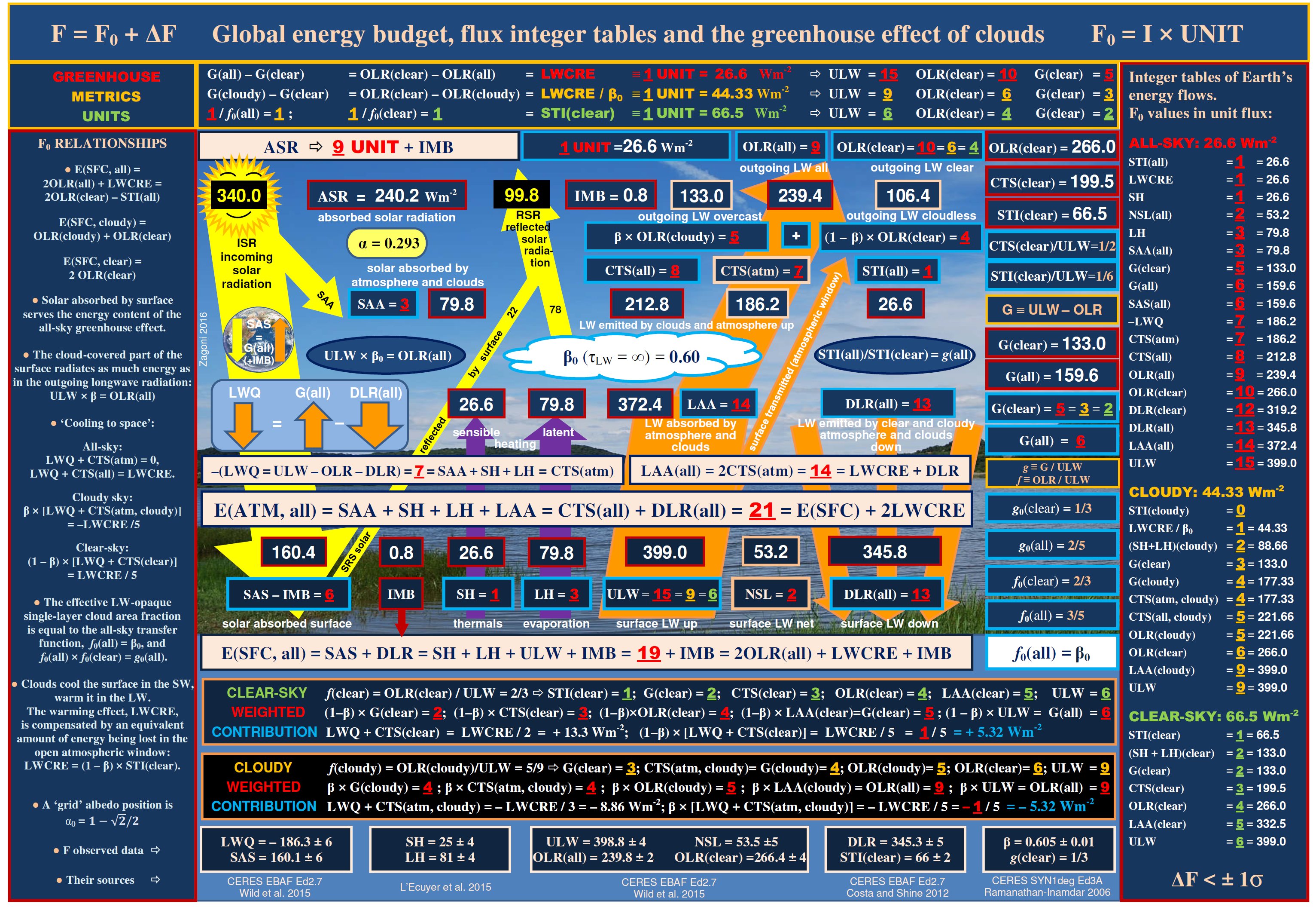 Click to enlarge. Bottom lines: the observed F values and their sources. Right column: F0 values as integer multiples of three different units. Top rows: the units and their interrelations. Left column: the three (all-sky, cloudy and clear-sky) surface energy balance equations. The validity of the 'cooling-to-space' approximation, and some relationships are detailed. 43.§.
Discussion
In
this section we examine several details of the energy budget. *** Let
our
first note be here that in our Poster we gave the explanation of
So far, in the Introduction, we have introduced this relationship from the closed-model perspective: the
LW energy being lost in the all-sky atmospheric window But
an opposite description is also possible, Clouds
cool the surface in the SW, warm it in the LW. The
physical principles in the background may be different, *** In
the followings we confine ourselves to the formal description of
the pattern;
44.§. Surface energy balance (Here we repeat some considerations already discussed in the Introduction.) It can be seen in the data that: the
all-sky energy income of the surface (absorbed
shortwave plus longwave downward radiation), E(SRF, all) = SAS(all) + DLR(all) = SH + LH + ULW = OLR(all) + OLR(clear). It
is easy to check this relationship on the latest published energy
budgets. Stephens
and L'Ecuyer 2015
has: SAS
= DSR – USW = 163 ± 6 W/m2 so OLR = 240 ± 4 W/m2, that
is, LWCRE
= 26.6 W/m2. E(SRF) = 2OLR(all) + LWCRE
= OLR(all) +
OLR(clear)
In the clear-sky subset the equation looks like: E(SRF, clear) = 2OLR(clear) and in the cloudy subset: E(SRF, cloudy) = OLR(cloudy) + OLR(clear). *** The simplest analogy to an E(SRF) = 2OLR atmosphere is the single-layer, SW-transparent, LW-opaque, non-turbulent 'glass-shell' greenhouse model: (John
Marshall - Alan Plumb: Atmosphere, Ocean, and Climate Dynamics.
Elsevier, 2008,
In this model, the atmosphere acts like a glass shell: there is no atmospheric shortwave absorption: SAA = 0, so all the solar energy is absorbed by the surface: ASR = SAS; and there is no escaping longwave transmission: STI = 0, therefore surface upward LW is completely absorbed by the shell: LAA = ULW – STI = ULW. This
energy radiates equally upward (out to space) and downward (to the
surface). So the surface energy balance reads: E(SRF) = ULW = ASR + DLR = 2OLR, As Marshall-Plumb (2008) put it:
Hence the left-hand side of Eq. (2-8) is E(SRF) = ULW, and the right-hand side is 2OLR. *** The "glass-shell" atmospheric model's periodic table looks like:
*** It can be seen from the data that, within ±0.5 W/m2, our partially opaque, partially cloudy and turbulent atmosphere, with the help of the longwave cloud effect, still maintains a 'quasi-opaque' greenhouse effect with E(SRF, clear) = 2OLR(clear) In
the all-sky case, E(SRF, all) = 2OLR(clear) – STI(all) but gained back by the longwave effect of clouds: E(SRF, all) = 2OLR(all) + LWCRE. Hence it is true that E(SRF, clear) = E(SRF, all) + LWCRE. Earth has a higher DLR and lower ULW than in the glass-shell model, and the difference in both cases is the turbulent flux: DLR(all) = OLR(all) + (SH + LH)(all) and ULW = E(SRF, all) – (SH + LH)(all). Adding them together we get: DLR(all) + ULW = OLR(all) + E(SRF, all). Now
let us realize that the surface energy balance equation of the
glass-shell case
which is the same as in the Earth's all-sky case: E(SRF, all) – DLR(all) = ULW – OLR(all) = G(all) .ULW = 2CTS (which is valid in our clear-sky) and LAA = 2CTS (which is valid in our all-sky) also stand. That is (conclusion here, but continued in Theory):
*** The
contribution of the cloudy part to the total
all-sky surface energy is and
the contribution of the clear-sky part is * 47.§. A major consequence for the atmosphere:
* 48.§.
Here
we examine how the abosrbed solar radiation, ASR, is distributed into the clear-sky and cloudy parts. The data we use are from CERES EBAF: ASR(all) = 240 W/m2 ASR(clear) = 287 W/m2 from here, with ASR(all) = β × ASR(cloudy) + (1 – β) × ASR(clear) we have ASR(cloudy) = 209 W/m2. Absorbed solar radiation in the all-sky mean is partitioned as β
× ASR(cloudy) + (1 – β) × ASR(clear)
= 0.6 × 209 + 0.4 × 287 = 125.4 + 114.8 W/m2; the
cloudy part of the
climate system absorbs 5.3 W/m2 more, the cloudless part 5.3 W/m2
less solar energy * Partition into atmosphere and surface: ASR(all) = SAA(all) + SAS(all) = 240 W/m2 = 160 + 80 W/m2 ASR(clear) = SAA(clear) + SAS(clear) = 287 W/m2 = 72 + 215 W/m2 ASR(cloudy) = SAA(cloudy) + SAS(cloudy) = 209 W/m2 = 85 + 124 W/m2. It
can be seen that: in
the all-sky average, one-third
of absorbed solar radiation is being absorbed by the atmosphere and
clouds, SAA(all) = ASR(all)/3 SAS(all) = 2ASR(all)/3. * According
to the data, SAS(all) = G(all). *** 49.§. Solar
absorption by the surface, SAS(all) is partitioned as the
cloudy part of the surface absorbs 5.8 W/m2
less, the cloud-free part 5.8 W/m2 more solar energy *** Reflected solar radiation: Reflected
solar radiation over the cloud-free areas, according to CERES
EBAF, is RSR(clear) = 52.6 W/m2, *** 50.§. NSL Net
surface longwave radiative cooling, NSL = ULW – DLR, under
clear
skies is ULW
– DLR(clear) = 79.8 W/m2, its value under clouds is NSL(cloudy) = 35.47 W/m2. Their area-weighted values are 31.92 W/m2 and 21.28 W/m2; their ratio is 3/2. *** 51.§. Turbulent fluxes Non-radiative cooling of the surface in the all-sky mean is
(SH + LH)(all) = 106.4 W/m2 = 4 LWCRE. Its value under clear skies is (SH+LH)(clear) = 5LWCRE = G(clear) = 133 W/m2; and under clouds is (SH+LH)(cloudy)
= 2 UNIT(cloudy) = 2LWCRE/β = G(cloudy)/2 = 88.66 W/m2.
Their
area-weighted quantities are the same, 88.66 × 0.6 = 53.2 W/m2 = 2 LWCRE = NSL(all). The total net cooling of the
surface is partitioned into the clear and the
cloudy part, separately, cool non-radiatively G(all) = 3 NSL(all) = 6 LWCRE. * It
can be seen that in
the all-sky mean,
Under the cloud deck, in the cloud-surface cavity, evaporation is the dominant effect, convective heat transport is small, or zero, in average. An interesting sub-case can be deduced from the SH(cloudy) = 0 approximation. Within this approximation, we would have: (SH + LH)(cloudy) = LH(cloudy) = 88.44 W/m2 = 2 LWCRE/β , hence, from SH(all) = LWCRE = 26.6 W/m2 and LH(all) = 3 LWCRE = 79.8 W/m2, we get SH(clear) = LH(clear) = 66.5 W/m2. That is,
*
52.§. Let us continue the clear-cloudy decomposition of the LW fluxes (G, LAA, DLR, CTS). The all-sky greenhouse effect as a weighted sum, G(all)
= β × G(cloudy) + (1 – β) × G(clear), and (1 – β) × G(clear) = 53.2 W/m2 = 2 LWCRE = NSL(all). *** 53.§. Longwave
atmospheric absorption in the cloudless
atmosphere is LAA(clear)
= 5 UNIT(clear) = ULW – STI(clear) = 332.5 W/m2, and
in the
cloudy subset LAA(cloudy) = ULW = 9 UNIT(cloudy) = 399 W/m2. The clear sky contribution is 332.5
× 0.4 = 133.0 W/m2 = G(clear), and
the cloudy contribution is *** 54.§. Downward
longwave radiation occupies
the position of DLR(all) = 13 LWCRE. and
in the cloudy subset The
clear-sky contribution to the all-sky global average is 319.2 × 0.4 = 127.68 W/m2 and in the cloudy subset 363.53 × 0.6 = 218.12 W/m2. DLR(clear)
is less than 5 LWCRE with 5.32 W/m2, DLR(all)
can be decomposed in the following way: = 133.0 + 79.8 + 133.0 = 345.8 W/m2,
but in the clear-sky subset there is an energy transfer from the surface to the atmosphere: LAA(clear) – DLR(clear) = 13.3 W/m2 = LWCRE/2, which results in a global average contribution of (1 – β) × LWCRE/2 = LWCRE/5 = 5.32 W/m2, and the opposite under clouds, with β × LWCRE/3 = LWCRE/5 = 5.32 W/m2. Therefore the actual composite cloudy/clear flows of DLR(all) are: DLR(all)
= [G(clear) + LWCRE/5] +
β × G(clear)
+ [G(clear) –
LWCRE/5] = (133.0 + 5.32) + 79.8 + (133.0 – 5.32) W/m2.
See also the calculation of CTS below. *** 55.§. The
cooling-to-space (upward atmospheric emission) flux element is
CTS(atm) = 199.5
× 0.4 + 177.33 × 0.6 = LAA(all)/2. This
relationship was first displayed numerically in the Trenberth and
Fasullo (2012) diagram, This
equality expresses the fundamental energetic fact that LAA(all) + 2LWQ = 0. *** 56.§. Here we examine in some detail the "Cooling-to-space approximation" The approximate equality of the cooling-to-space flux gradient and the total spectral cooling rate of an atmospheric column for several levels and gases in a number of climatic situations (tropical, mid-lattitude, arctic) was first observed under clear sky conditions by Rodgers
and Walshaw (1966): The computation of infra-red cooling rates They say: the
“radiation
cooling at any level is due to the exchange of radiation between that
level and
["its
importance cannot be overstated", said Goody and Yung 1989, An interesting question arises: how
much are the corresponding flux elements
"cooling-to-space"
(CTS), the same as "emitted by atmosphere upward" in the
Trenberth-diagrams; the
latter flux element being equal to the LW energy entering from below
less that
leaving it above and below, LWQ = ULW – OLR – DLR. Since
the (c) term (radiation between the different atmospheric levels) is
evidently zeroed out in the integral, For the global averagewe found that CTS(atm) = –LWQ and CTS(all) + LWQ = LWCRE. This all-sky mean value is a result of compenstaion between the clear and the cloudy parts of the atmosphere. It
is evident also that under clear-skies, the (b) term, IR radiation
exchange term with the ground, cannot be zero: How much is it? Its value in the clear-sky part is, as show in our poster: LWQ + CTS(clear) = [ULW – OLR(clear) – DLR(clear)] + CTS(cler) = [399.0 – 266.0 – 319.2] + 199.5 = –186.2 + 199.5 = 13.3 W/m2 = LWCRE/2; its contribution to the global average is (1 – β) × [LWQ + CTS(clear)] = LWCRE/5 = 5.32 W/m2. * In the cloudy part, with similar calculation, LWQ + CTS(atm, cloudy) = [ULW – OLR(cloudy) – DLR(cloudy)] + CTS(atm, cloudy) = [399.0 – 221.66 – 363.53] + 177.33 = – LWCRE/3 = 8.87 W/m2, and its contribution to the global averge is β × [LWQ + CTS(cloudy)] = – LWCRE/5 = – 5.32 W/m2. *Hence their sum in the all-sky mean is really zeroed out: LWQ + CTS(atm) = 0. We regard this equality as one of our important results which stands on its own. *** From the equality LWQ + CTS(clear) = LWCRE/2, * using the terms from their definition: * LWQ = ULW – OLR(clear) – DLR(clear) ULW = LAA(clear) + STI(clear) OLR(clear) = CTS(clear) + STI(clear) * it can be deduced that LWQ + CTS(clear) = LAA(clear) – DLR(clear), hence the right-hand side is also equal to LWCRE/2: * LAA(clear) – DLR(clear) = LWCRE/2. * Therefore a hypothetic equality LWQ + CTS(clear) = 0 would mean LAA(clear) = DLR(clear), but
in
reality, according to the theory and the observed data, That's
why DLR(clear) doesn't have the same position of No. 5 as LAA(clear) in
the clear-sky structure; DLR(clear) = 12 × 26.6 W/m2 = 319.2 W/m2. This is a correction to our paper, where, based on earlier studies, we incorrectly inserted DLR(clear) into position No.5 of the clear-sky table. * We
think the
importance of the above relationships in the global energy budget is
that The equalities of LAA(clear) = DLR(clear) + LWCRE/2 and LAA(all) = DLR(all) + LWCRE serve as fundamental pillars of the stability of Earth's global energy balance; see our diagram. *** 57.§. The formalism given by the flux periodic tables helps us to recognize some further interrelations. The
cloud-covered part of the surface emits the
energy f(all) serves as a mapping of ULW into OLR(all), and by the given cloud area fraction, ULW
is mapped into OLR(all)
Evidently the clear-sky mapping function gives ULW × f(clear) = OLR(clear). The all-sky greenhouse function gives ULW × g(all) = G(all). Note that the mapping of OLR(clear) into G(all) is: OLR(clear) × f(all) = G(all), therefore g(all) = f(clear) × f(all), see also below. * 58.§.
The ratio of the clear and
cloudy areas is equal to the clear-sky transfer function: (1 – β0) / β0 = 0.4 / 0.6 = 2/3 = f(clear) , and
the ratio of the cloudy area to the total surface (3/5) β0 = f(all). Finally,
the ratio of the clear area to the total surface (2/5) (1 – β0) = g(all) ..
Ramanathan and Inamdar (2006): The radiative forcing due to clouds and water vapor. 59.§. * From
f(all)
= β × f(cloudy) + (1 – β) × f(clear)
- the ratio of the all-sky and the cloudy units is β0 = f0(all) = 3/5, and - the ratio of the cloudy and the clear-sky units is f0(clear) = 2/3; therefore g0(all) = f0(all) × f0(clear). The connection between the different units can be established as:
LWCRE = β × LWCRE(cloudy) + (1 – β) × LWCRE(clear), STI(all) = β × STI(cloudy) + (1 – β) × STI(clear)
where,
by definition,
and
hence
*
60.§ Albedo A paper on "The albedo of Earth" G. Stephens, D. O'Brien, P. Webster, P. Pilewski, S. Kato, Jui-lin Li 2015, Rev Geophys 53:141-163
found a "surprising", "dramatic" hemispheric symmetry (“the Northern and Southern Hemispheres reflect the same amount of sunlight within ~ 0.2 Wm/2”) and
a "remarkably
small"
interannual
variability of reflected solar radiation (RSR) so two questions are given there: . "Is the hemispheric symmetry purely coincidental?" . "Is the albedo of Earth highly constrained?" . Let us first realize that the ratio of absorbed and incoming solar radiation is ASR/ISR
= 240.2/340 = sin 45° = √2/2, hence the albedo, RSR/ISR
= α =
1 – sin 45° = 1 – √2/2
= 0.293 seems constrained, symmetrical and very stable. The probability for an incoming photon to be reflected rather than absorbed is therefore RSR/ASR = (1 – sin 45°) / sin 45° = √2 – 1.
*** *** It
is worthwhile to recall here that the CERES EBAF Ed2.8 all-sky
reflected solar radiation, (Differences between the successive versions of Ed2.6, Ed2.7 and Ed2.8 are within ± 0.5 W/m2.) The weighted contribuition of the clear and the cloudy part to this total outgoing shortwave flux is: clear: (1 – β) × RSR(clear) = 0.4 × 52.4 = 21 W/m2 cloudy: β × RSR(cloudy) = 0.6 × 131 = 78.7 W/m2, coherent
with 22 W/m2 surface upward SW (USW) flux and 79 W/m2
atmosphere + cloud reflection, Parallel to the longwave flux, where the blanketing effect of clouds was calculated as LWCRE = OLR(clear) – OLR(all), the shortwave cloud radiative effect, or the shielding effect of clouds, can be formed as SWCRE = RSR(clear) – RSR(all) = – 47.3 W/m2. In the longwave, the gross cloud effect was calculated as LWCRE / β = OLR(clear) – OLR(cloudy); similarly, SWCRE / β = RSR(clear) – RSR(cloudy) gives the gross shortwave cloud radiative effect, with a value of –47.3 / 0.6 = –78.8 W/m2, as it ought to be. Finally, and also evidently, 78.8 / 0.6 = 131 W/m2 is the nominal (per area) cloud contribution to the all-sky mean. *** Having these data, let us repeat here the computation of the surface energy balances given elsewhere: 52.4 W/m2 clear-sky reflection from 340.0 W/m2 incoming solar radiation leaves ASR(clear) = 287.6 W/m2 absorbed solar radiation in the clear-sky part of the globe. From this, 243.9 W/m2 reaches the surface and 29.7 W/m2 is reflected from the surface, therefore SAS(clear) = 214.2 W/m2 is the nominal solar radiation absorbed by the surface in the clear-sky part. Hence the clear-sky solar atmospheric absorption is SAA(clear) = 73.4 W/m2. Having LW down (clear-sky) at the surface in the same data set DLR(clear) = 316 W/m2, the energy absorption by the surface in the clear-sky part is the sum of the SW and LW absorbed radiation: E(SRF, clear) = SAS(clear) = DLR(clear) = 214.2 + 316 = 530.2 W/m2. This data set gives LW TOA clear-sky radiation OLR(clear) = 265.7 W/m2. Therefore: E(SRF, clear) = 2OLR(clear) – 1.2 W/m2. The
'box model' surface balance equation is fulfilled, *** In possession of the clear-sky and all-sky data, the cloudy values can be computed. ASR(cloudy) = [ ASR(all) – (1 – β) × ASR(clear)] / β = 209 W/m2 SAA(cloudy) = [ SAA(all) – (1 – β) × SAA(clear)] / β = 84 W/m2 SAS(cloudy) = [ SAS(all) – (1 – β) × SAS(clear)] / β = 125 W/m2. The cloudy surface energy balance equation is then: E(SRF, cloudy) = SAS(cloudy) + DLR(cloudy) = = 2OLR(clear) – LWCRE / β = = 2OLR(cloudy) + LWCRE / β = = OLR(clear) + OLR(cloudy). Evidently
the highly regulated clear-sky and the cloudy-sky solar absorptions and
reflections Isn't the "buffering effect" beyond the "remarkably small interannual variability", as mentioned by the albedo-paper, is based on the surface energy budget constraint of the box model? 61.§. It seems also that even β, the single-layer IR-opaque equilibrium cloud are fraction, is constrained at β = f0(all) = 3/5. For our case, let us put the question in this form: Is
the energy budget of Earth highly constrained? and,
at the surface, the sum of energy flows in the balance equation are
restricted
to the energy flows at TOA: * 62.§. Evaporation, clouds: stabilizing feedback? It
seems
that evaporation and clouds play stabilizing role on the whole system: 'energy matrix' elements, but there are a lot of others, equally important, and energetically perhaps much more rigid relationships: 2G(clear) = OLR(clear) 2CTS(clear) = ULW 2CTS(atm) = LAA(all) LWQ = – CTS(atm) SAS(all) = G(all) OLR(all) = ULW × beta, STI(all) = LWCRE f(all) = beta etc., most importantly the E(SRF) = 2OLR + LWCRE, which bounds the surface energies to that of at TOA. Therefore do not think that they all are regulated by the evaporation/cloud feedback. They, all together, are strictly constrained by the whole system of overall energetic restrictions. These are digital ('quantum') states, 'grid positions' in the chrystal structure sense. Of course one may describe the vibrations of the atoms around their lattice position in a chrystal, or the stability of the electron orbit around the atomic nucleus as controlled by 'feedbacks', but we don't regard it is the most adequate conceptual framework. *** This
is actually not a "climatic" problem, it is a physical
question: 63.§. Clear-sky
pattern
We presented the clear-sky periodicity in this form: STI(clear) = One G(clear) = Two CTS(clear) = Three OLR(clear) = Four LAA(clear) = ULW – WIN(clear) = Five ULW = Six * A rather technical question may arise here: Are the annual global mean clear-sky and all-sky surface upward radiations equal? The answer is not necessarily yes, but we recline here upon Kato et al. (2013), Table 4, who shows an equality. In case of new data, this can be refined. * DLR(clear) is measured by BSRN (Baseline Surface Radiation Network, Ohmura et al.) and given as DLR(clear) = 319 (±9) W/m2 (see also Stephens et al 2012.), its position in the clear-sky pattern is DLR(clear) = 5 STI(clear) – LWCRE/2. It has a position in the all-sky structure as TWELVE UNIT(all) = 12 LWCRE = 319.2 = 12 × 26.6 W/m2 = 319.2 W/m2, showing the inter-connectedness of the clear and the all-sky values through the globally determined and controlled relationship of f(all) = β = 0.6. *** Conclusion here:
*** 65.§. If
each element is quantized, and the energy budget is constrained, A recent presentation says:
(Trenberth
K, Fasullo J, Schuckmann K, Cheng L 2016: outgoing
longwave radiation is OLR(all) = 239.6 /m2, The ratio of OLR(all) = 9 units and ULW = 15 units must be f0(all) = OLR(all) / ULW = 3/5, hence the equilibrium surface radiation belonging to the observed OLR is ULW = 239.6 / 0.6 = 399.33 W/m2. This is higher with 1.23 W/m2 than the measured surface radiation. Earth's surface must warm, ocean heat content must grow, to reach the equilibrium. Based on the found pattern we state: Imbalance is not a consequence of "increased GHGs"; We cannot expect energy imbalance form heat-trapping GHGs; Surface warms until ULW increases to match OLR /f0(all) = 5OLR(all)/3; The most fundamental measure that cimate is changing is the difference of ULW and OLR(all)/0.6 . *** Let us notice: The opening slide of the above Princeton-presentation does not list H2O as infrared radiation-emitting gas (perhaps because it is not an 'increased' GHG, but belongs to 'feedbacks and complexities'):
*** The above presentation refers to a CLIVAR-research project. Here is the original CLIVAR logo; it assumes an imbalance from heat-trapping GHGs:
* And here is our central equality projected on it, showing the TOA < — > SRF interconnection:
The energy budget at the surface is NOT a free variable of GHGs. According to the observed data, it is completely determined by the energy budget at TOA. As
always, Readers are asked to check these equalities themselves, *** We infer that present-day imbalance is not a long-term, ever-growing process. It
is a consequence of a temporary (natural or triggered) fluctuation
around the Time-scale
of these fluctuations is not yet known.
66.§.
LWCRE =
STI(all)
One of the most important elements of the structure is the above relationship. How could we understand this? What is the direction of causation? Clouds have two opposite effects on the system: a shielding effect in the SW, and a blanketing effect in the LW. The former cools, the latter warms the surface, therefore the latter is called the greenhouse effct of clouds. LWCRE => STI(all) Let us approach the question from the energy minimum principle: let us assume that the system seeks its possible lowest energy state. From this point of view, the shielding effect is 'useful', the blanketing effect is 'harmful'. Now the above equality can be read this way: The surface gets rid of the superfluous cloud warming effect by an equivalent amount of energy being lost in space through the open atmospheric window. * STI(all) => LWCRE But the reading in the opposite direction is also possible. If the system wants to maximize its energy content (trying to behave like a 'closed system'), then the spectral regions being transparent (because of the molecular absorbing properties) should be somehow made opaque. The system solves the problem of closing the open atmospheric window by the LW cloud effect; by the help of LWCRE it gains back the energy being lost in STI(all). * LWCRE <=> STI(all) The most probable solution is the mutual determination: the clear-sky transparency depends on the water vapour content, as well as the cloud amount. If STI(clear) is determined as OLR(clear)/4, and OLR(all) is given by ASR, then LWCRE is connected to STI and beta, in both directions: LWCRE = OLR(clear) – OLR(all) = (1 – β) × STI(clear) = (1 – β) × OLR(clear)/4. In this system, every element is being mutually determined by all the others – that is, by the whole structure. *** Below we try to map the way of the incoming energy into the particular units and describe the interconnections among the elements.  67. §
Energy
flow routesThe flow of the incoming solar radiative energy (ISR = 340.0 W/m2) through the climate system can be depicted as follows. RSR = ISR × (1 – sin 45°) = 99.8 (± 0.2) W/m2 is reflected, ASR = ISR × sin 45° = 240.2 (± 0.2) W/m2 is absorbed in the surface-atmosphere system. 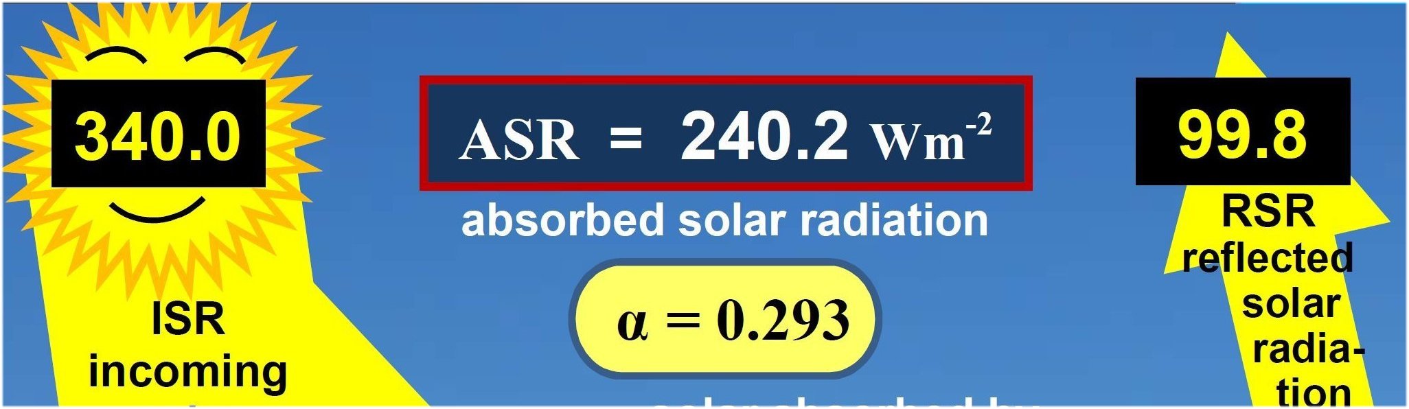 *** ASR (9) = SAA (3) + SAS (6) ASR, in the all-sky global average, is broken into three equal parts. One part is being absorbed by the atmosphere and clouds (SAA(all) = 79.8 W/m2):  the remaining two is absorbed by the surface (SAS(all) = 160.4 W/m2; imbalance: 0.8 W/m2): 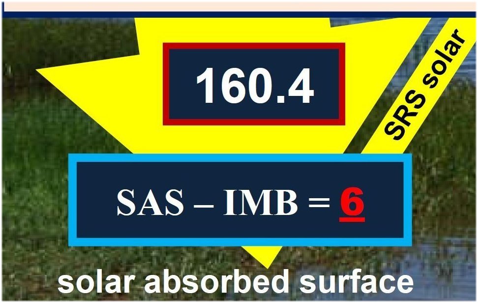 *** 68. §
SAS(all) (6) = G(all) (6) The latter is being transformed into longwave radiation in the surface, serving the energy content of the all-sky greenhouse effect: SAS(all) – IMB = G(all) = ULW – OLR(all) = 6 UNIT(all) = 159.6 W/m2 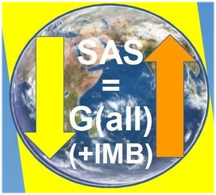 *** G(all) (6) = NSL(all) (2) + (SH + LH)(all) (4) This amount of energy is again being devided into three equal parts. One part of it serves as net surface longwave radiative cooling, NSL(all) = ULW – DLR(all) = 2 UNIT(all) = 53.2 W/m2, 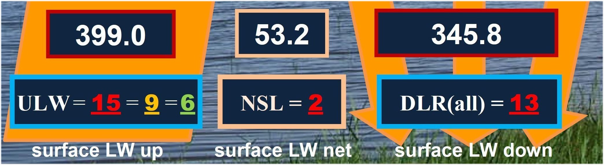 the remaining two parts serve as surface non-radiative cooling: (SH + LH)(all) = 4 UNIT(all) = 106.4 W/m2 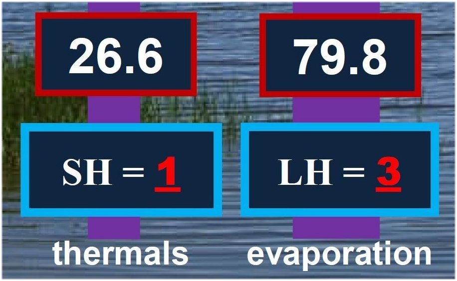 *** NSL(all) (2) = LWCRE (1) + STI(all) (1) NSL(all) itself is a sum of two equal quantities: NSL(all) = LWCRE + STI(all) 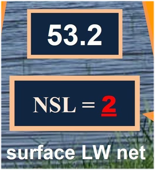 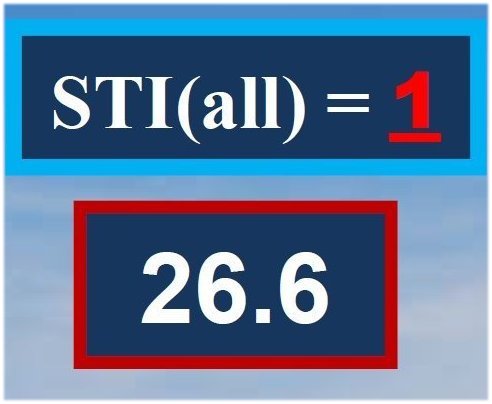  *** LWQ (-7) = ULW (15) – OLR(all) (9) – DLR(all) (13) The atmospheric all-sky greenhouse effect, G(all), augmented by one unit of longwave cloud effect, LWCRE, offers the energy content of upward atmospheric emission, called also 'cooling-to-space', CTS(atm), and is equal to the total net atmospheric column cooling, LWQ: 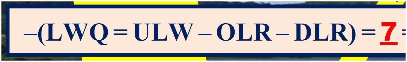 *** LWQ (-7) = G(all) (6) – DLR(all) (13) G(all) + LWCRE = CTS(atm) = – LWQ = – (ULW – OLR(all) – DLR(all)) = 7 UNIT(all) = 186. 2 W/m2 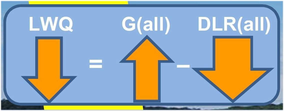 *** - LWQ (7) = SAA (3) + (SH + LH)(all) (4) This longwave loss of the energy in the atmosphere is being balanced by the non-radiative atmospheric energy incomes (shortwave absorption plus turbulent heating): – LWQ = SAA(all) + (SH + LH)(all) = 7 UNIT(all) = 186.2 W/m2. *** – LWQ (7) = CTS(atm) (7)  *** CTS(atm) (7) + LWCRE (1) = CTS(all) (8) One LWCRE upward, added to CTS(atm) gives CTS(all), and one LWCRE downward, substracted from LAA(all), leads to DLR(all): CTS(atm) + LWCRE = CTS(all) = 8 UNIT(all) = 212.8 W/m2, 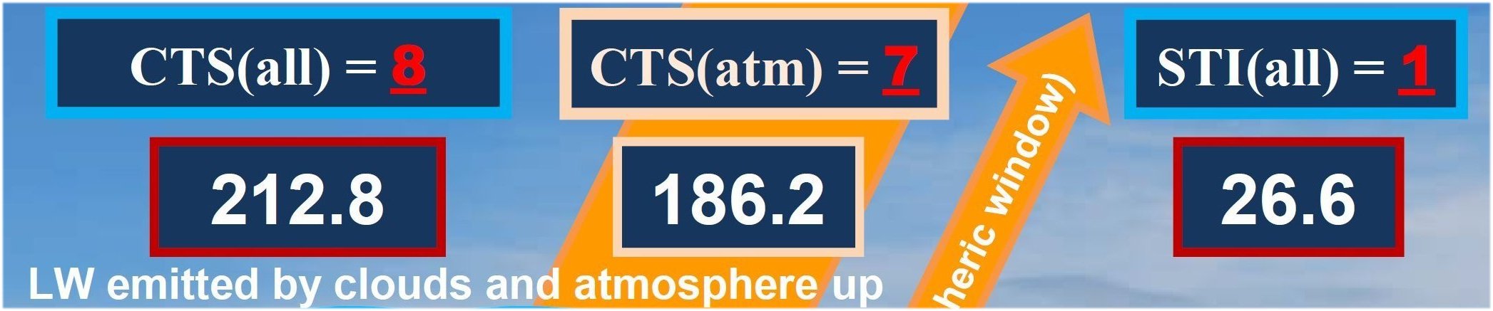 *** LAA(all) (14) – LWCRE (1) = DLR(all) (13) LAA(all) – LWCRE = DLR(all) = 13 UNIT(all) = 345.8 W/m2 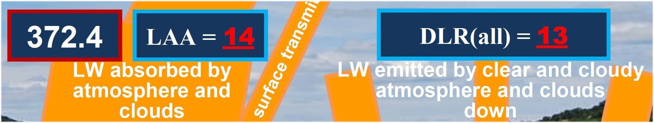 *** LAA(all) (14) = ULW (15) – STI(all) (1) = 2 × CTS(atm) (7) The energy in the upward emission of the surface, ULW, is being absorbed by the atmosphere, except the transmitted (escaping) part, STI(all): LAA(all) = ULW – STI(all) = 14 UNIT(all) = 2 CTS(atm) = 372.4 W/m2  *** E(ATM, all) (21) = CTS(all) (8) + DLR(all) (13) = = SAS(all) (3) + (SH + LH)(all) (4) + LAA(all) (14) This total energy of upward and downward atmosheric emissions is being supported by the solar atmospheric absorption and turbulent heat, together with longwave atmospheric absorption: CTS(all) + DLR(all) = SAS(all) + (SH + LH)(all) + LAA(all) = 21 UNIT(all) 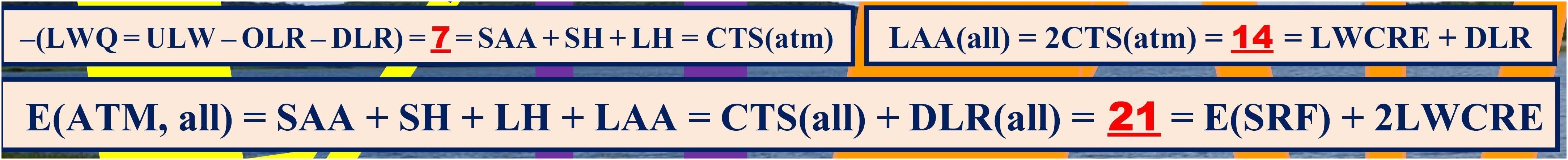 *** 69. §
E(SRF, all) (19) = SAS(all) (6) + DLR(all) (13) = ULW (15) + (SH + LH)(all) (4) = 19 UNIT(all) = 2 × ASR (9) + LWCRE (1) At the surface, downward longwave radiation, added to surface absorbed solar radiation, DLR(all) + SAS(all), give the energies in the surface balance equation, and being balanced by the sum of radiative and non radiative cooling of the surface: E(SRF, all) = DLR(all) + SAS(all) = ULW + (SH + LH)(all) = 19 UNIT(all) = 505.4 W/m2 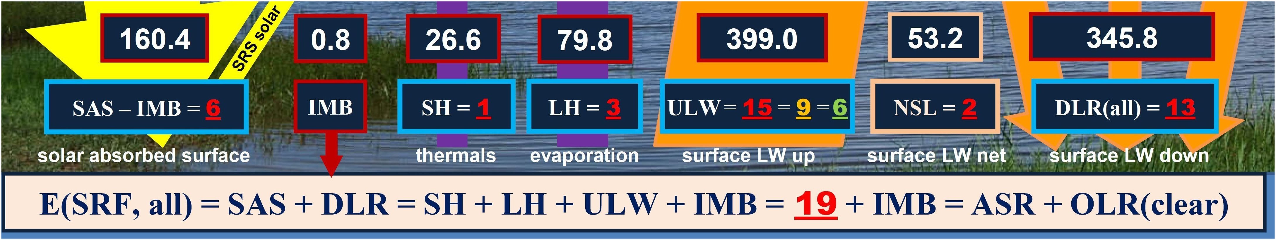 *** CTS(all) (8) + STI(all) (1) = CTS(atm) (7) + NSL(all) (2) = OLR(all) (9) At TOA, CTS(all), joining to STI(all) (which comes from the surface), provide the energy content of outgoing longwave radiation: CTS(all) + STI(all) = OLR(all) = 9 UNIT(all) = 239.4 W/m2 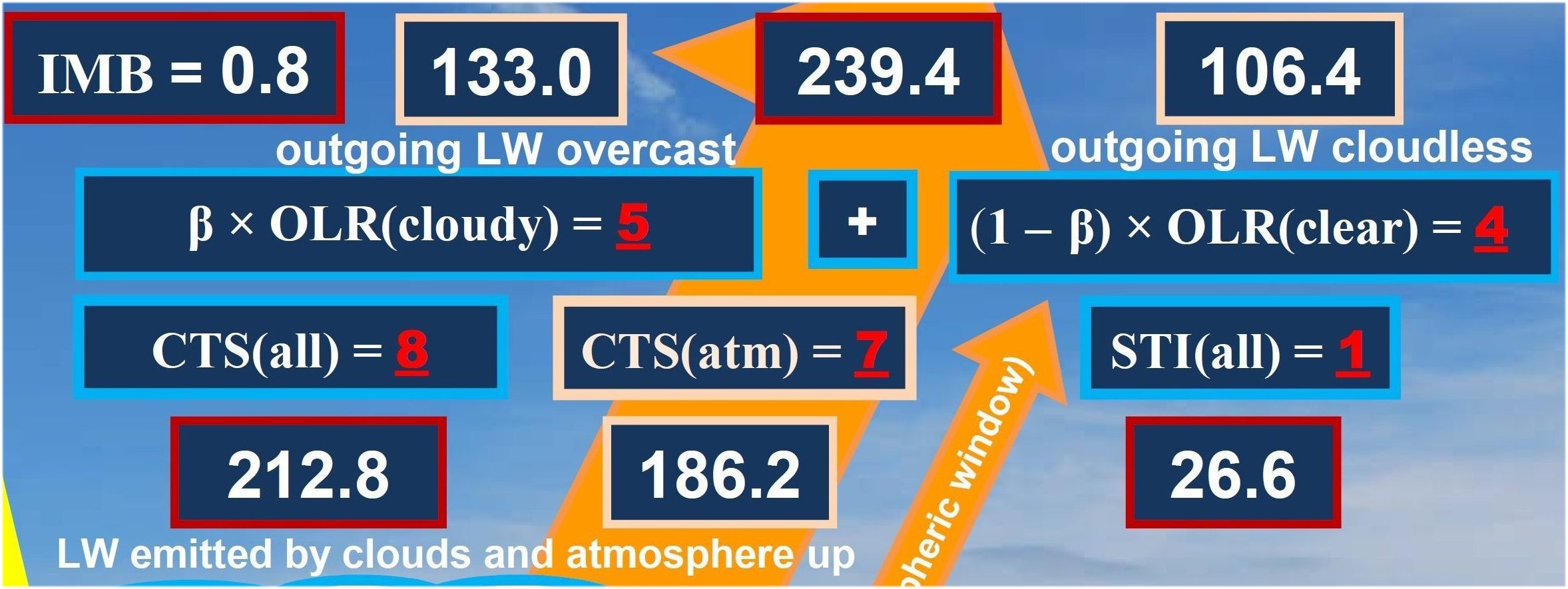 *** β = 0.6 According to NASA CERES Aqua and Terra satellite observations for the past fifteen years, our best information today about the total cloud area fracion is (as we cited already above): 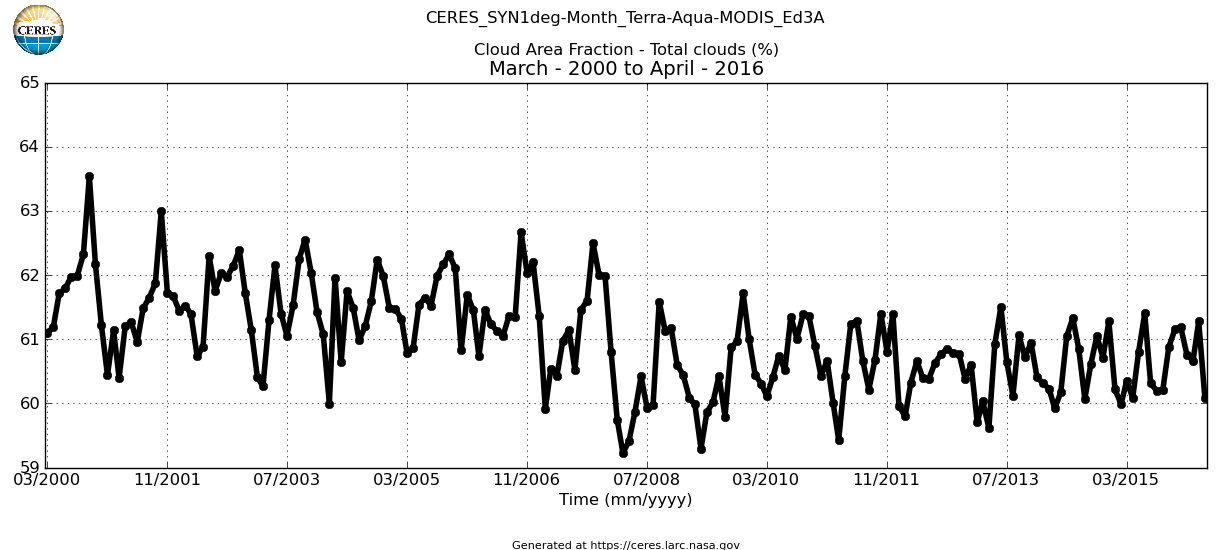 For the past six or seven years, its shows a fluctuation between typically 60 and 61%, around about 60.5 %. We regard the effective IR-opaque single-layer equilibrium cloud area fraction as β0 = 0.60:  *** ULW(15) × β (3/5) = OLR(all) (9) With this value, we have: The cloud-covered part of the surface, ULW × β, radiates the amount of OLR(all), 399 × 0.6 = 239.4 W/m2  *** ULW (15) × (1 – β) (2/5) = G(all) (6) and the clear-sky part radiates ULW × (1 – β), which is G(all): 399 × 0.4 = 159.6 W/m2. *** f0(all) = OLR(all) (9) / ULW (15) = 3/5 = β0 (0.6) Hence the cloud area fraction, β, serves also as the all-sky transfer function, f(all) = OLR(all)/ULW = 3/5;  *** f0(clear) = OLR(clear) (10) / ULW (15) = 2/3 the ratio of the clear- and the cloudy parts, (1 – β)/β = 0.4/0.6 = f(clear) = 2/3 as the clear-sky transfer function; and the ratio of the clear-sky part to the total surface, (1 – β) = 0.4 = g(all) as the all-sky greenhouse function 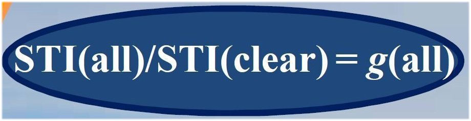 *** 70.
§
Now the all-sky greenhouse effect is connected to G(clear) as the clear-sky outgoing longwave radiation is connected to OLR(all): through the value of longwave cloud effect, LWCRE,  and the cloudy greenhouse effect to its clear-sky counterpart as the clear OLR to the cloudy one:  These are our units of measure, or our  Augmented with the third unit, which is the measure under clear skies,  we have also the relationships between the three units. *** 71.
§
Now three of the basic elements of the energy flow system, ULW, OLR(clear) and their difference, G(clear), can be expressed with all of these units: 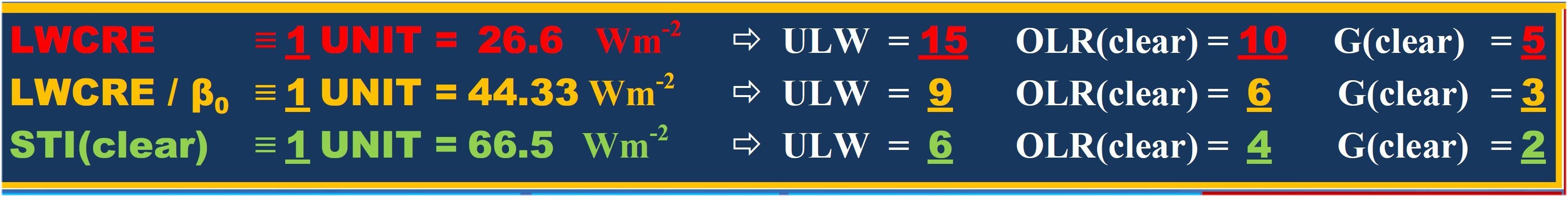 That is,   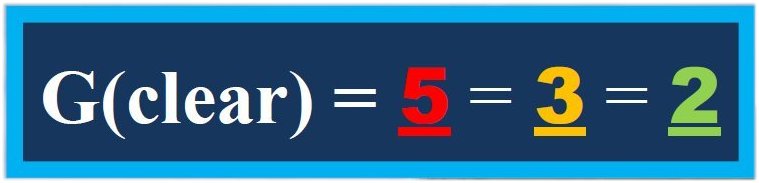 . .With the observed values, 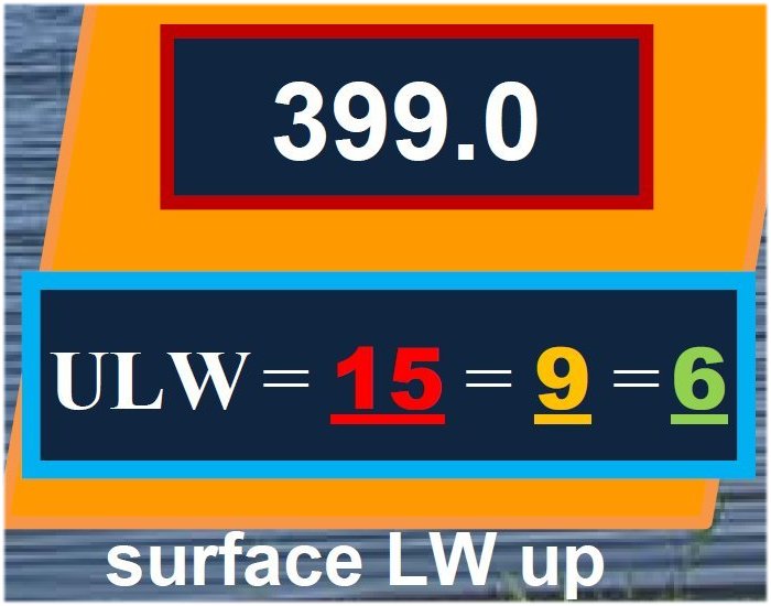 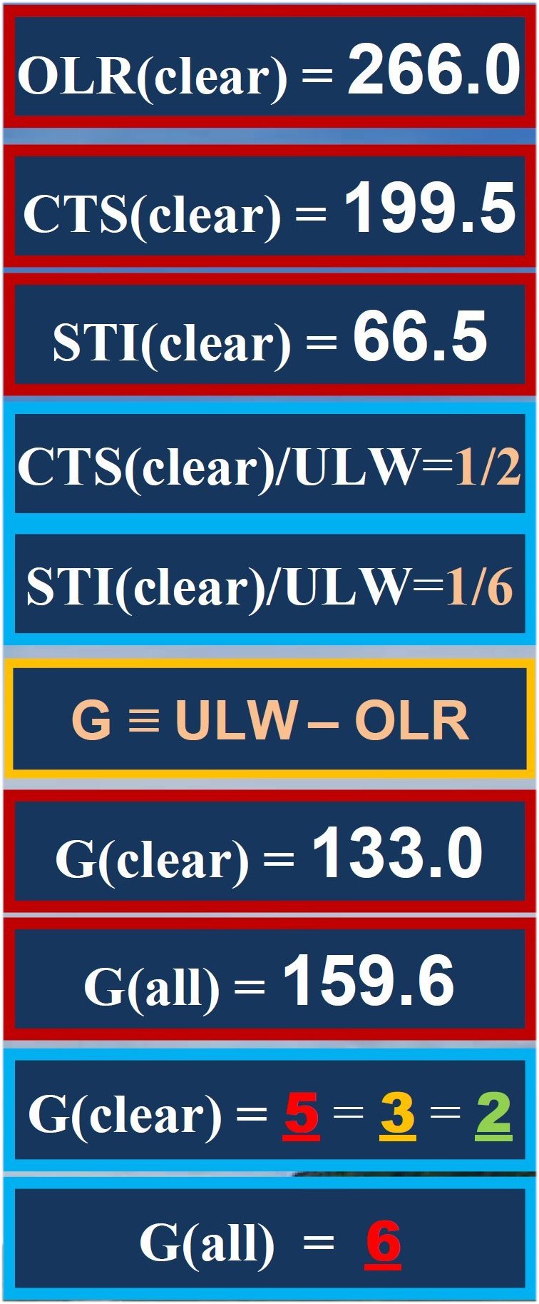 *** All the other observed F fluxes can be written as  where  N is an integer between one and fifteen, and the units are given above. With these, we get three periodic tables of fluxes in three different units: 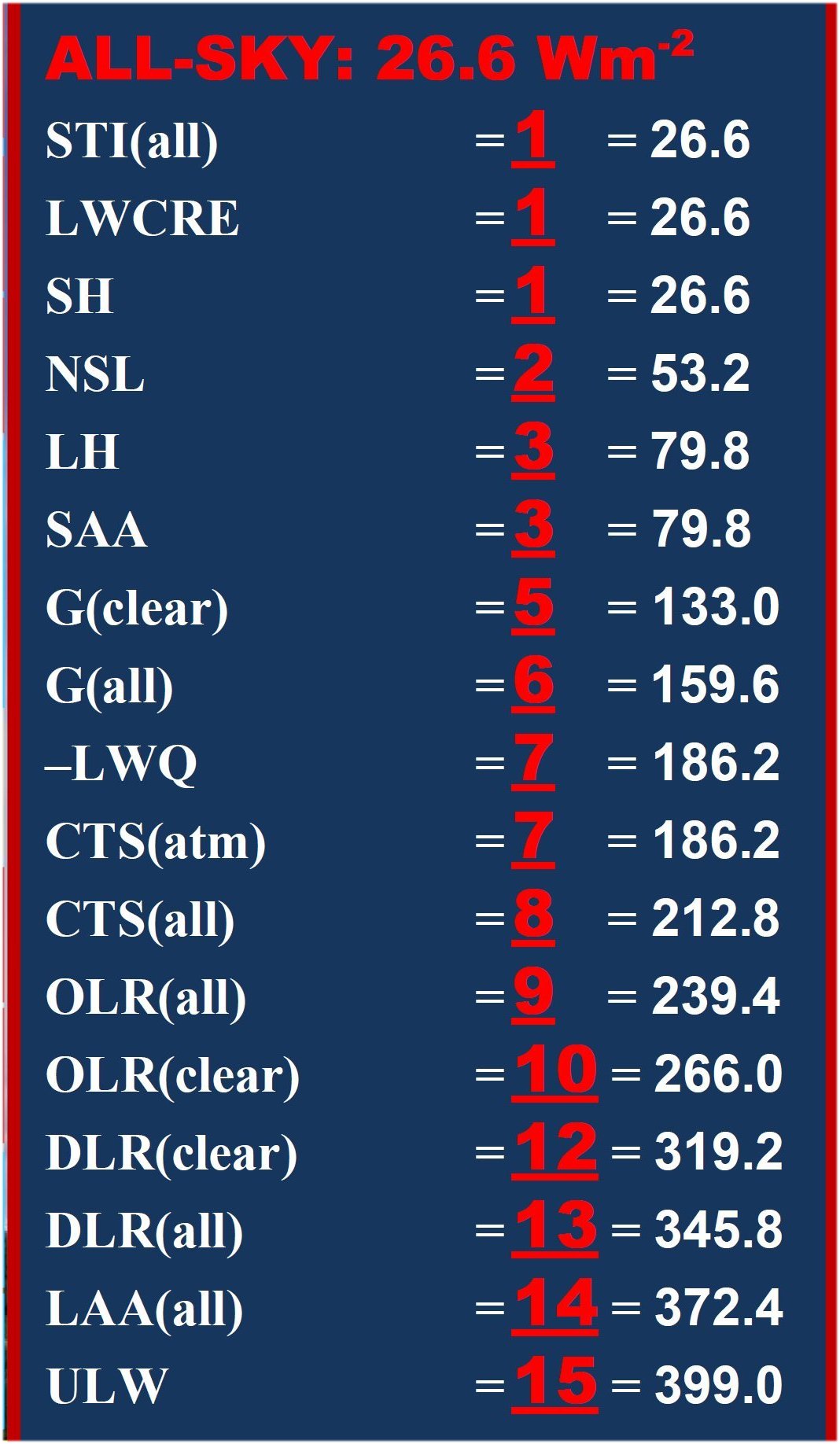 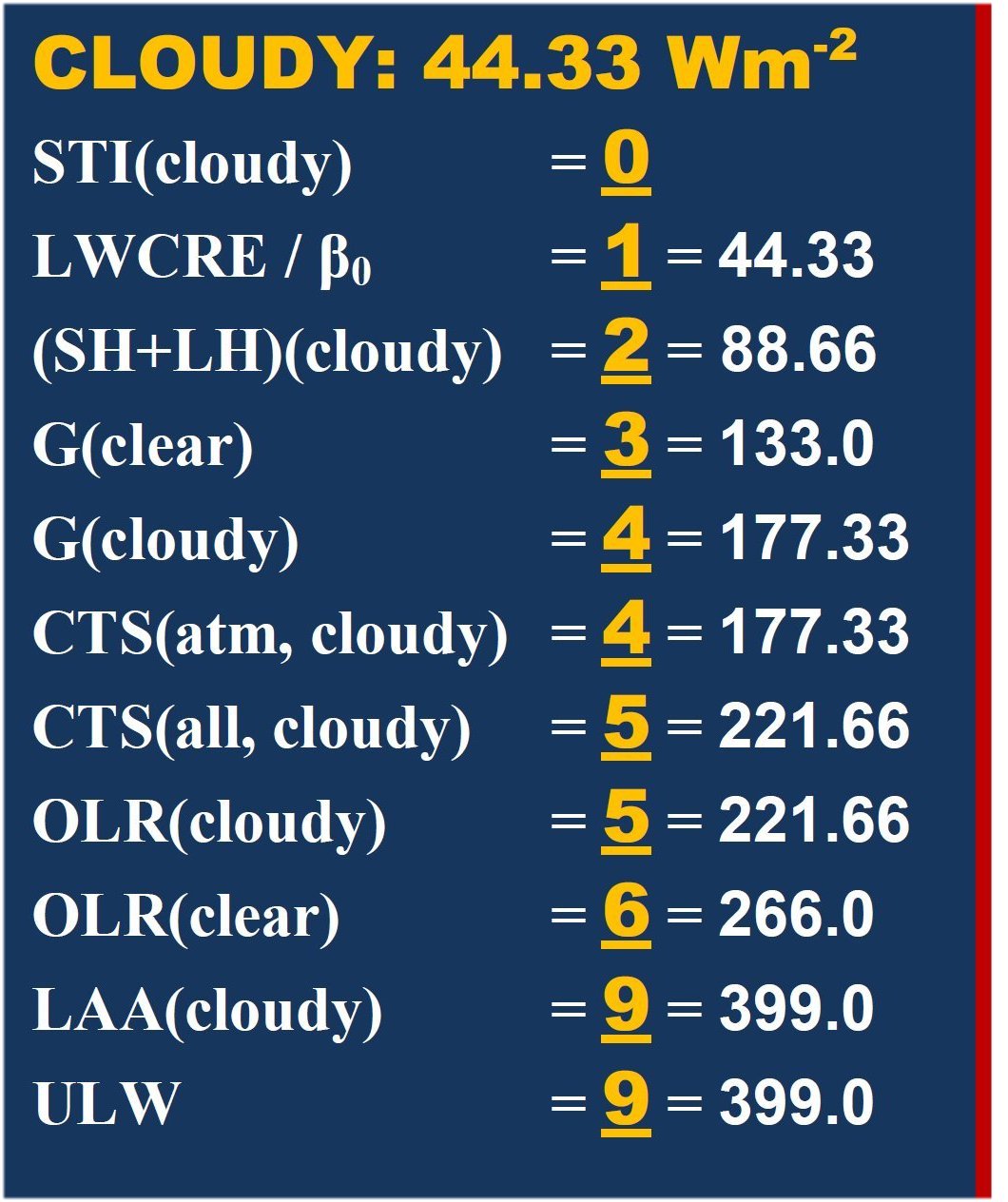 *** 72. §
The observed all-sky (and where indicated, clear-sky) values are given at the bottom of our poster: 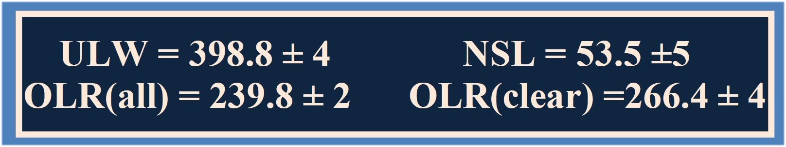 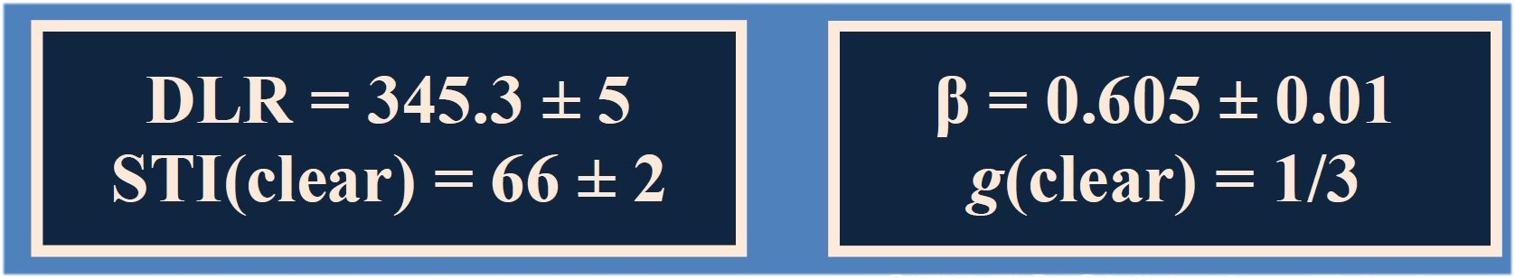  The Δ difference between the observed F values from their above-given F0 quantities is much smaller than one standard daviation:  *** 73.
§
Let us note: we have started the section with the observation that the absorbed solar radiation in the all-sky system, ASR(all) = 240.2 W/m2, is being devided into three equal parts (one part is absorbed by the atmosphere, SAA(all) = 79.8 W/m2, and two parts are absorbed by the surface, SAS(all) = 160.4 W/m2). Now we should add: the solar radiation absorbed in the clear-sky part, ASR(clear) = 287 W/m2 (data from CERES EBAF), is being devided into four pieces: one is absorbed in the atmosphere (SAA(clear) = 72 W/m2, and three is absorbed by the surface: SAS(clear) = 215 W/m2 (see e.g. Wild 2015b). These latter quantity, added to the downward longwave radiation, take up the total surface energy under clear skies: E(SRF, clear) = SAS(clear) + DLR(clear) = 215 + 319 = 534 W/m2, with a data-uncertainty of ± 5 W/m2. This energy income is balanced by the radiative and non-radiative energy release of the surface: E(SRF, clear) = ULW + (SH + LH)(clear) = 399 + 133 W/m2 The two important points here are that the surface energy is conneted to that of TOA as: (a) E(SRF, clear) = 2 OLR(clear) ; and the turbulent surface cooling is equal to the greenhouse effect: (b) (SH + LH)(clear) = G(clear), far within to the data observation error. *** 74.
§
Now the Cathedral of our Heavens above our heads seems to be carefully designed and very well-constructed; it is built from blocks or bricks of the following size: The outgoing longwave radiation in the clear-sky part is being split into FOUR equal parts: OLR(clear) = 4 UNITS(clear) = 4 STI(clear) = 4 × 66.5 W/m2 = 2 G(clear) = 2 × 133.0 = 266.0 W/m2;  the outgoing longwave radiation in the cloudy part is being split into FIVE equal parts: OLR(cloudy) = 5 UNITS(cloudy) = 5 LWCRE/ β = 5 × 44.33 W/m2 = 221.66 W/m2, with G(clear) = 3 × 44.33 W/m2 and G(cloudy) = 4 × 44.33 W/m2 = 177.33 W/m2  and the outgoing longwave radiation in the all-sky mean is being split into NINE equal parts: OLR(all) = 9 UNITS(all) = 9 LWCRE = 9 × 26.6 W/m2 = 239.4 W/m2, with G(clear) = 5 × 26.6 W/m2 and G(all) = 6 × 26.6 W/m2 = 159.6 W/m2;  and every other flux is being built from these elements. The size of these bricks is predestined by the size of the corresponding OLR, and does not depend on the atmospheric chemistry. On the contrary, the total effective atmospheric IR-absorber composition, including the concentration and distribution of water vapor, seems to be regulated by the design of the energy flows. 75. §
*** The King among these radiations is atmospheric downward longwave emission to the surface, DLR, called also "back-radiation"; once it was proposed to 'another measure of the greenhouse effect' (Inamdar and Ramanathan 1997, On monitoring the atmospheric greenhouse effect from space. Tellus 49B: 216-230). A paper dealing solely with DLR says in its Introduction: "It has been understood for some time that changes to the strength of the greenhouse effect are fundamental to our understanding of the climate of earth and how it can change (Arrenhius 1896; Callendar 1938; Kasting 1989). Increases in greenhouse gases like CO2 induce a warming of the surface and lower atmosphere. The increase in water vapor that follows a warming results in a further strengthening of the greenhouse effect by increased emission of radiation from the atmosphere to the surface that induces even more warming. This is the essence of the positive water vapor feedback that occurs through the connections between temperature, water vapor, and emission of infrared radiation (e.g., Held and Soden 2000)." G. Stephens, M. Wild, P. Stackhouse, T. L'Ecuyer, S. Kato, D. Henderson (2012): The Global Character of the Flux of Downward Longwave Radiation Journal of Climate, 25: 2329-2340 We think that while the paper presents correct observed data about the clear-sky and all-sky DLR, none of the above statements are supported by the data. *** IPCC 2007 WGI AR4 Chapter 02 says: "Philipona et al. (2004) found an increase in the measured longwave downward radiation at the surface over the period from 1995 to 2002 at eight stations over the central Alps. A significant increase in the clear-sky longwave downward flux was found to be due to an enhanced greenhouse effect after combining the measurements with model calculations to estimate the contribution from increases in temperature and humidity." We think that temporal and local changes in the clear-sky downward flux cannot be attributed to an enhanced greenhouse effect. Or, if its measured value still increases, it is because it was below of its equilibrium position. The stability to the strength of the global greenhouse effect is fundamental to the climate of earth, and both the clear-sky and the all-sky downward atmospheric emission sit very sharply in their given grid position: The above paper from Stephens et al. says DLR(all) is between 344 and 350 W/m2. Stephens et al. (2012) give DLR = 345.6 W/m2, its pattern position in our diagram is 345.8 W/m2. We show DLR(all) as a sum of three components: 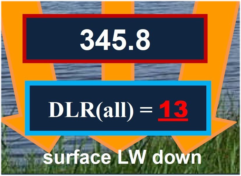 That is the quantity which is expected (by the prevailing theory) to undergo the largest increase of all radiative fluxes over this century: 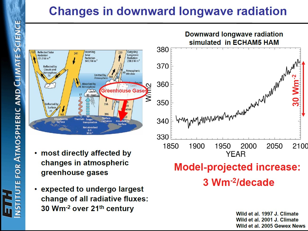 Wild M (2011) BSRN: Science and Operations Update AOPC-XVI, WMO, Geneva, Feb. 8 2011. As said, its observed value today, as proposed by Stephens et al. (2012), is 345.6 W/m2: it occupies its grid position within 0.2 W/m2. The clear-sky F0 value is DLR(clear) = 319.2 W/m2 (= 12 LWCRE); Stephens et al. give an observational DLR(clear) = 319 W/m2 to it; F and F0 again within Δ = 0.2 W/m2. The cloudy value is DLR(cloudy) = 363.53 W/m2 = DLR(clear) + LWCRE/β. The three components shown in our diagram are: From the clear-sky part: 0.4 × 319.2 = 127.68 W/m2 = G(clear) – LWCRE/5, from the cloudy part: 0.6 × 363.53 W/m2 = 0.6 × (319.2 + LWCRE/β) = G(clear) + 3LWCRE + LWCRE/5. That is, the symmetrical decomposition, DLR(all) = 13 UNITS(all) = (5 + 3 + 5) UNITS(all) = DLR(all) = G(clear) + β × G(clear) + G(clear) is modified into DLR(all) = [2 UNITS(clear) – LWCRE/5] + 3 UNITS(all) + [3 UNITS(cloudy) + LWCRE/5] = DLR(all) = [G(clear) – LWCRE/5] + β × G(clear) + [G(clear) + LWCRE/5]. It is sitting sharply in its prescribed all-sky global mean position of 13 LWCRE. That's why we think that the above-proposed increase cannot (and will not) happen. (For the source of the asymmetry, see more details in the "Cooling-to-space approximation" section above, 56. §) 76.
§
*** The Queen of all these energies, the greenhouse effect itself, being defined as the difference of surface emission and outgoing radiation, G = ULW – OLR, can also be understood as follows: — In the clear-sky part, it is equal to the non-radiative surface energy release: G(clear) = (SH + LH)(clear) = 133.0 W/m2, and equals also to TWO clear-sky units (2 × 66.5 W/m2); — In the cloudy part, it is equal to the double of the non-radiative energy flows: G(cloudy) = 2 (SH + LH)(cloudy) = 2 × 88.66 W/m2 = 177.33 W/m2, being equal to FOUR cloudy units (4 × 44.33 W/m2) (in the cavity of the surface-cloud box, it seems something like thermals up plus thermals down); — and in the all-sky mean, it equals to the sum of the surface non-radiative and net radiative cooling: G(all) = (SH + LH)(all) + NSL(all) = 106.4 + 53.2 = 159.6 W/m2, being equal to SIX all-sky units (6 × 26.6 W/m2). Note that the surface, in the all-sky mean, cools non-radiatively twice as much as radiatively:
= +
The longwave energy content of G(all), gained from the solar absorption by the surface, SAS(all), in the all-sky mean is completely counter-balanced by the surface non-radiative plus net radiative cooling. The contribution of the cloudless part to the all-sky mean is 0.4 × 133.0 = 53.2 W/m2, which is TWO all-sky units; the contribution of the cloudy part to the all-sky mean is 0.6 × 177.33 = 106.4 W/m2, which is FOUR all-sky units; so the G(all) = SIX all-sky mean is again being devided into three equal parts: one is coming from the clear atmosphere, and two from the cloudy. 77.
§
That's
why we think that the increase of the greenhouse effect, as predicted
by the prevailing theory (cited in our Introduction from Wild 2015a),
will not happen: *** 78.
§
Isn't it interesting? The ratio of surface net-radiative and non-radiative cooling in the cloudless area is 3/5 = f(all), (with NSL(clear) = 79.8 W/m2 = 3 UNIT(all)) and (SH+LH)(clear) = 133.0 W/m2 = 5 UNIT(all)), while this ratio under clouds is 2/5 = g(all), (with NSL(cloudy) = 35.47 W/m2 = 4/5 UNIT(cloudy)) and (SH+LH)(cloudy) = 88.66 W/m2 = 3 UNIT(cloudy)). The weighted contributions to the non-radiative cooling from the clear and the cloudy parts are equal: (1 – β) × (SH + LH)(clear) = β × (SH + LH)(cloudy) = NSL(all) 0.4 × 133.0 = 0.6 × 88.66 = 53.2 W/m2, and the weighted contributions to the net-radiative cooling from the clear and the cloudy parts are: (1 – β) × NSL(clear) = 0.4 × 79.8 = 31.92 W/m2, β × NSL(cloudy) = 0.6 × 35.47 = 21.28 W/m2, their ratio is 3/2. *** Generally, the weighted contributions of the clear and the cloudy parts of the atmosphere to the all-sky mean are:  *** Let us repeat it for all flux elements, with the periodic tables. Clear-sky values, and their weighted contribution to the all-sky mean: *** Cloudy sky values, and their weighted contribution to the all-sky mean: 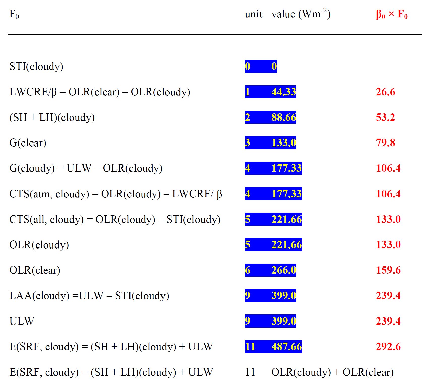 And finally, once more, the all-sky [(1 – β) × CLEAR) + β × CLOUDY] mean: 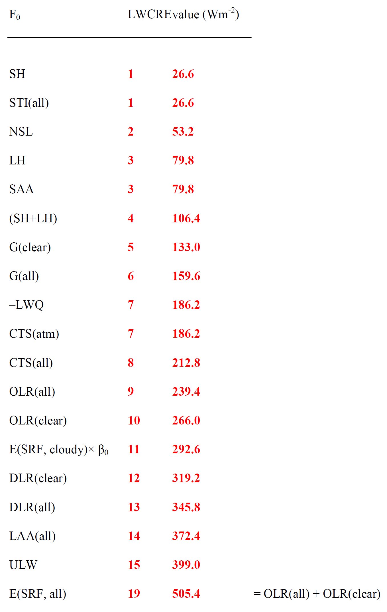 *** That's how, we think, the absorbed solar radiation is partitioned into the found units, creating the wonderfully designed composition we experience. *** 79.
§
Our
Sun seems to be
quite happy with these new results. 80. §
TheoryIt is evident that in the present state of the work, we cannot give a complete conceptual descripition, a new hypothesis or theory on how our climate system might work that mainatins the given patterns, periodicities and structure. So our comments will be necessarily inconclusive, and we just repeat here what we have said in the Introduction. The best analogy we can offer is the "box model", or the "closed system analogy", as treated above in the Introduction, and in the first section of the Discussion. In the simple SW-transparent, LW-opaque, non-turbulent "glass-shell" atmosphere the surface energy was uniquely determined by, and double of, the incoming energy: 81. §
E(SRF, glass-shell) =
ULW(glass-shell) = 2OLR(glass-shell).In the real case of the partially SW-transparent, partially LW-opaque and partially cloud-covered Earth, the surface energy is still uniquely determined by the energy flows at TOA, in the form of E(SRF, clear) = 2OLR(clear) , 82. §
E(SRF, all) = 2OLR(clear) –
STI(all) = 2OLR(all) + LWCRE.and E(SRF, cloudy) = OLR(cloudy) + OLR(clear). The question appears, how the system solves the problem of becoming LW-opaque, that is, of "closing the atmospheric window". * Costa and Shine (2012) note that about "one-tenth of the OLR originates directly from the surface". This also means that only about one-fifteenth of the surface emission reaches directly to space. That is, our atmosphere is 'almost-closed'. Kiehl and Trenberth (1997) when calculating LWCRE (their Fig. 2) note that "the largest effect of clouds on the outgoing longwave flux is in the atmospheric window (8–12 micron)" Their values were STI(all) = 40 W/m2 and LWCRE = 30 W/m2. Now we have seen that with STI(clear) = 66.5 W/m2 of Costa and Shine and β = 0.6 of CERES, it is true that STI(all) = (1 – β) × STI(clear) = LWCRE. Now the answer may lay in the 83.
§
STI(all) = LWCRE equality, which says that the surface transmitted LW energy being lost in the open atmospheric window is given back to the surface by the equivalent amount of energy in the cloud greenhouse effect. In a "leaky" atmosphere the energy content of STI(all) is "lost in space" from a surface viewpont; but in a "closed by clouds" atmosphere the energy content of STI(all) is gained back by the greenhouse effect of clouds. In this sense, the energetic role of the partial cloud cover in the LW is to close the atmospheric window — that is, to make the system non-transparent in the infrared. *** 84. §
In another frasing:As the atmosphere is not saturated for the LW-absorption (becouse of the molecular absorption properties, there is a transparent region in the H2O, as well as in the CO2-spectrum), the LW-blanketing effect of the clouds is called into the sceen to help to keep the energy "in". This kind of "closed" character is reflected in the simple (and easily controllable) relationships of 2 G(clear) = OLR(clear) saying that the upwelling and downwelling LW energies in the clear-sky greenhouse effect utilize the entire amount of LW energy in the outgoing radiation; 2 CTS(clear) = ULW saying that the atmospheric upward emission in the clear-sky part is double of the surface energy; this equality maps the 2OLR = ULW glass-shell relationship, as OLR(clear) = CTS(clear) + STI(clear); 2 CTS(atm) = LAA(all) this one says that in the all-sky case, atmospheric LW absorption, which is ULW less STI(all), is double of the all-sky atmospheric upward emission: 2 [OLR(all) – STI(all) – LWCRE] = ULW – STI(all), that is, finally, 2 OLR(all) = ULW + 3 LWCRE and E(SRF) = ULW + 4 LWCRE = 2 OLR(all) + LWCRE. The same structure expresses the same content as in the closed "glass-shell" atmospheric model in our realistic, partially-transparent atmosphere, with "modulated" periodic tables. *** This "wave in a box" character seems to appear in the integer multiples of the internal fluxes: LWCRE = ONE STI(all) NSL(all) = TWO LWCRE, etc. and in all the presented internal integer ratios and proportions. As an analogy, in lack of a better explanation, should we call the propagating energy in the "box" a "wave", and N in the F = N × UNIT equation "wave number"? *** The conclusive statement here would be evidently to show how this result can be deduced from some first principles — say, from the principle of least action. Part of the deduction may go like this: One
of the most universal physical laws is the
principle
of energy minimum: a ball at the bottom of a potential hole, or the
cooling of
a hot stove in a cold room. The hot surface of the Earth cools two
different ways: by turbulent (latent + sensible) heat release, and by
radiative
cooling. The most efficient (maximized) latent cooling maximizes the
atmospheric water vapor content (greenhouse gas), leading to the
narrowest
(tightest) atmospheric window (lowest IR transparency). The most
efficient
radiative cooling of the surface into the space requires the widest
atmospheric
window (highest IR transparency). On our aqua-planet, there is an
evident equilibrium between the two opposite constraints: the ratio of
the
turbulent/radiative cooling is predetermined by physical constants:
sea-flux/Planck-flux must be a given, fixed value.
***
Closing
remarks85. §.
"It
is unequivocal
that anthropogenic increases in the well-mixed greenhouse gases
(WMGHGs) have substantially enhanced the greenhouse effect, and the
resulting forcing continues to increase."
– says the very first sentence of the Executive Summary of IPCC 2013 Working Group I AR5, Chapter 8. [In: Climate Change 2013: The Physical Science Basis. Contribution of Working Group I to the Fifth Assessment Report of the Intergovernmental Panel on Climate Change. Cambridge University Press] We hope we have shown here that it is NOT unequivocal that anthropogenic increases in WMGHG's have at all enhanced the greenhouse effect. We didn't want to introduce a counter-hypothesis here; we did not insist or assert anything speculative. We just state that, according to the observed data, the greenhouse effect sits very stably in its 1/3 and 2/5 clear-sky and all-sky pre-fixed 'grid' value. Our purpose was to show these 'observations' about the characteristics of the published energy budget data, and to share our contemplations about them to trigger a discussion.
87. §
Conclusions HARMONIA PLANETARIS Stations of a cooperation Pictures of an exhibition Deduction of the basic characteristic of Earth's energy budget in 4 steps:  I.
Schematic model
of a planet closed into a greenhouse The surface energy flows are unequivocally predetermined by the incoming energy: E(SRF) = ASR + DLR = ULW = 2OLR = 2ASR. f = OLR/ULW = 1/2 g = G / ULW = (ULW – OLR) / ULW = 1/2. * II. Schematic model of the clear-sky part of the Earth's atmosphere (semi-transparent in SW and LW, turbulent): In the cloud-free part
of the atmosphere the reflected solar radiation is less, SAA + SAS = ASR > OLR Further, DLR is higher than OLR, ULW is lower than 2OLR DLR > OLR ULW < 2OLR There is turbulent heat transfer from the surface into the atmosphere, SH + LH > 0. And still, according to CERES data: OLR(clear) = 266 W/m2 ASR(clear) = 287 W/m2 SAA(clear) = 74 W/m2 SAS(clear) = 213 W/m2 DLR(clear) = 319 W/m2 E(SRF, clear)
= SAS + DLR = ULW + SH + LH = 2OLR(clear) * III.
Schematic model
of the cloudy part of the Earth's atmosphere
In the cloudy part of
the atmosphere the reflected solar radiation is more, SAA + SAS = ASR < OLR, There is no longwave surface transmission through the clouds: STI(cloudy) = 0. DLR > OLR, ULW < 2OLR, SH + LH > 0. And still ... E(SRF, cloudy) = SAS + DLR = ULW + SH + LH = OLR(cloudy) + OLR(clear)* IV.
Schematic model
of the all-sky atmosphere of
Earth 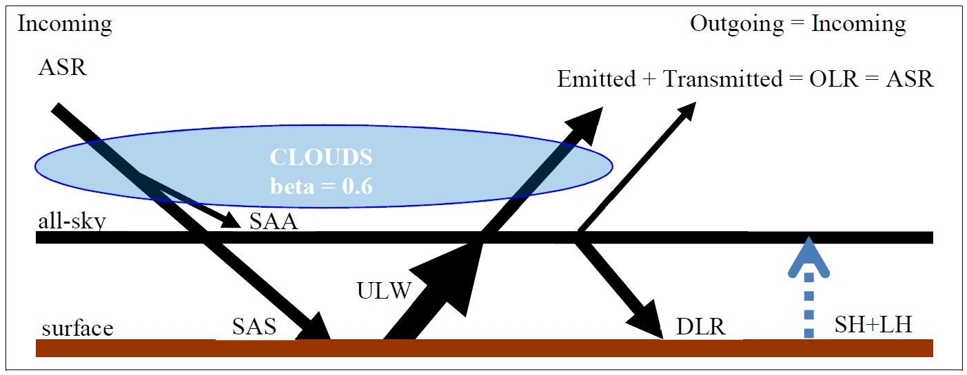 In
the all-sky mean, Earth maintains a delicate equilibrium on the
planetary level The cloud area fraction
is also part of the cooperation which
finally leads to a = 2OLR(clear) – STI(all) = 2OLR(all) + LWCRE as shown in more detail in our energy budget poster. 88. §
* As a result of the 'closed-into-a-glass-shell-greenhouse' model, the energy flows show a discrete, integer-multiple characteristic. We presented the observed values of the F flux terms in Earth’s global energy budget as F = F0 + ΔF, where F0 = N × U; N is an integer, U is a unit flux and ΔF is a deviation. Based on the published data we have shown that: with the flux unit U = LWCRE, the elements fit into an all-sky pattern; with U = LWCRE/ β into a cloudy pattern, and with U = LWCRE/(1 – β) = STI(clear) into a clear-sky pattern. The ΔF deviations of the observed F values from their F0 pattern positions are smaller (typically within ±2 W/m2) than ±1σ range (typically ± 4W/m2) of data uncertainty. *** According to the data, in the global average, the sum of the energy flows at the surface seems to be unambiguously determined by the energy flows at TOA, within an imbalance, separately for the clear, cloudy and the all-sky case: E(SRF, clear) = 2OLR(clear) E(SRF, cloudy) = OLR(clear) + OLR(cloudy) E(SRF, all) = OLR(clear) + OLR(all) . *** From the 'leaky closed model' we can deduce the actual interconnections. In the closed case, both the transfer and the greenhouse function have a value of 0.5. On Earth, where STI(all) / OLR(clear) = 1/10, i.e., one-tenth of the clear-sky emission is a 'lost-in-space' surface radiation through the all-sky atmospheric window, it follows that f(all) = 5/10 + 1/10 = 0.6 g(all) = 5/10 – 1/10 = 0.4 And: if the clear-sky atmospheric transparency is 1 – ε(clear) =1/6 and the all-sky transparency is 1 – ε(all) = 1/15, then the (1 – β) × 1/6 = 1/15 equation determines an IR-opaque cloud area fraction of β = 3/5 = 0.6. From here, with the all-sky planetary emissivity of OLR(all) / ULW = 9/15 = 0.6 we have for the clear-sky value of the transfer and greenhouse functions: f(clear) = 9/15 + 1/15 = 2/3, g(clear) = 6/15 – 1/15 = 1/3. *** The longwave-regulated β0 = f0(all) = 3/5 energetic requirement then maintains a cooperation between the clouds and the surface, leading to a constrained ASR / ISR = 240.4 /340.0 = sin 45° = √2/2 shortwave absorption ratio and a symmetric planetary albedo of α0 = 1 – sin 45° = 1 – √2/2 = 0.293. . 89.§.
ConsequencesIf this pattern is not purely coincidental but represents reality, then the whole-number units maintain the given vulgar fractions, ratios and relationships, and prevent the global state from continuous shifts and smooth internal reorganization. As long as the all-sky flux values are multiples of LWCRE = OLR(all)/9, it can be inferred that – The clear-sky and all-sky greenhouse factors occupy their exact pattern positions at g(clear) = 1/3 and g(all) = 2/5; hence – Elevated (enhanced) greenhouse effect is not possible. [ The term "enhanced, elevated, increased greenhouse effect" is used as in the IPCC (2013) WGI AR5 Chapter 02 and Chapter 08; and would mean that ULW grows without increasing ASR or OLR. ] OLR(all) is made up from 9 blocks or bricks or quanta, OLR = 9 LWCRE, ULW is made up from 15 blocks or bricks or quanta: ULW = 15 LWCRE. They can move only together; the equilibrium all-sky transfer function is f(all) = OLR/ULW = 9/15 = 3/5, therefore the equilibrium all-sky greenhouse factor is g = 1 – f = (ULW – OLR)/ ULW = G(all)/ULW = 2/5 = 0.4, and no smooth tendency or shift is possible. Only vibrations, natural or externally triggered, annual or decadal or centennial or millennial or longer variability is allowed around the 'grid' (F0) value. * If the structure described here is true – and it seems to us that all the fluxes occupy their F0 position precisely –, than ULW, and G, and g cannot increase without an increase in ASR (or OLR). * That's why we say that the equilibrium greenhouse sensitivity is zero for increasing CO2. Note: The latter does not mean that CO2, H2O do not have IR emission/absorption. It means only that, according to the published CERES data, all the fluxes are sitting in their pre-determined position. Therefore, the whole atmospheric temperature and IR absorption/emission structure (including the water vapor amount, greenhouse effect magnitude and cloud formation) is created, organized, prescribed and maintained by the albedo - cloud area fraction - SW absorption - LW emission (and evaporation, precipitation, atmospheric IR transparency, window value etc.) structure. * 90. §
Hence, based on the above considerations,
we can state that:- The equilibrium greenhouse sensitivity (EGS) is zero; - The equilibrium climate sensitivity (ECS) might contain only secondary (indirect) effects; - 'Global warming' is not greenhouse warming, - "Holding the increase in the global average temperature to well below 2 °C above pre-industrial levels", as the Paris Climate Agreement says, assumes an invalid direct connection between CO2 and global temperatures. We may infer further from here that: The model-predicted gradual 30 W/m2 increase in the flux of DLR to the end of this century, as a function of changing surface air temperature forced by a 1% per year increase in CO2, as shown in the Supplementary Information to the Stephens et al. (2012) Nature Geoscience paper, is not possible: 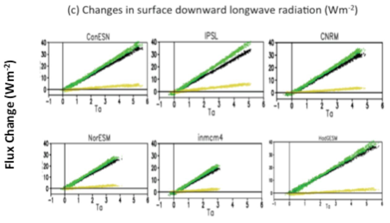 Stephens et al. 2012 NGEO1580 Suppl Inf Figure S2 (c) The main consequence of our results can be given in the verifiable form of a forecast: if the structure we have presented in our paper and in this website is true; if the flux values continue to occupy their grid position as whole-number multiples of LWCRE; if LWCRE remains a brick being equal to one-ninth of OLR(all); if DLR remains to be built up from 13 bricks of LWCRE then the model-predicted smooth or gradual increase in DLR as a result of increasing CO2, as shown in a Wild 2011 WMO presentation will not happen: Slide #27 from the presentation M. Wild (2011) BSRN: Science and Operations Update 91. §
Key uncertainties Some
of the fundamental observable flux parameters are accurately measured
to accept their values, most notably the basic LW boundary fluxes: ULW,
OLR and DLR; their deviation from their grid position is within 1
W/m2.
SW fluxes are slightly less certain; and the turbulent fluxes, mainly sensible heat, are the most uncertain. The
computed fluxes depend on the atmospheric data base and the computer
code; the most essential parameter, clear-sky window flux can be
regarded as 66 ± 2 W/m2.
The largest source of uncertainty is the value of cloud area fraction. The
ISCCP (International Satellite Cloud Climatology Project) publishes
higher cloud area fractions than the CERES (Clouds and the Earth's
Radiant Energy System) observations. A frequently referred value is
67.5 ± 1.2 % from Rossow and
Schiffer (1999); some later
energy budget studies accepted this quantity when calculating the
all-sky atmospheric window as STI(all) = 66 × (1 – 0.675) = 21.5 W/m2
(see Trenberth and Fasullo 2012).
A current GEWEX study (Stubenrauch, Rossow, Kinne et al. 2013) refers to the ISCCP result as: "Global
total cloud amount (fractional cloud cover) is about 0.68 (±0.03), when
considering clouds with [SW] optical depth > 0.1. The value
increases to 0.74 when considering clouds with optical depth <
0.01
(e.g. CALIPSO) and decreases to about 0.56 when clouds with optical
depth > 2 are considered (e.g. POLDER)."
It is evident that very thin clouds (with visible optical depth < 0.01) might have IR optical depth < 1. The
CERES project from March 2000 to March 2016 has 62% cloudiness for the
first decade, then an average of 60.5% for the last seven or so years.
We
regard the single-layer IR-opaque effective cloud amound (area
fraction) as beta = 0.60, therefore our STI(all) = 66 × (1 – 0.6) =
26.4 W/m2 is higher than the one based on the ISCCP data.
Further
observational and modelling efforts are needed to have an objectively
established magnitude for this fundamental climate parameter.
92.§.
Questions
and
challenges- Variability: timescale and magnitude of possible fluctuations ("oscillations, vibrations") around the pattern (grid) positions? - Systematic deviations from the grid positions? - "Quantum jumps" between the grid positions ("ground state" vs. "excited states")? - Same global average with different regional, vertical and/or seasonal distributions? - Another stable global configuration? - Another eigenvalue for the albedo α0 = 1 – sin 45° = 1 – √2/2 = 0.293 ? - Another eigenvalue for the cloud area fraction β0 = f0(all) = 0.6 ? - Effects of increasing CO2? - If CO2 radiative forcing goes up, does this mean that H2O must go down? - Reaction of clouds (change in type, height and geographic distribution)? - Ice ages? The trigger of the interglacial-glacial transitions? - Where are the limits and the Achilles-heels of the stability of our climate? - If GW is not AGW, then which is the next most dangerous human influence? * 93. §
SummaryOur
results can be sorted into four different baskets,
each of them representing very specific types of constraints. All of the following relationships are based on published observational data. I. We showed that the energy flows at the Earth's surface are completely predetermined by the energy flows at TOA, and can be written as E(SRF, clear) = (SH + LH)(clear) + ULW = 2 OLR(clear) E(SRF, cloudy) = (SH + LH)(cloudy) + ULW = OLR(cloudy) + OLR(clear) E(SRF, all) = (SH + LH)(all) + ULW = OLR(all) + OLR(clear) = 2OLR(all) + LWCRE. For the latter, let us repeat it in quantitative form, in W/m2: E(SRF, all) = 106.4 + 399.0 = 239.4 + 266.0 = 2 × 239.4 + 26.6 . * The physical content of this equality may be expressed this way: The Earth's atmosphere is almost opaque in the infrared: only one-fifteenth of the surface upward longwave emission reaches TOA through the open atmospheric window. In the SW-transparent, LW-opaque non-turbulent closed glass-shell model, where all surface upward longwave emission is absorbed by the shell, the surface energy balance equation reads: E(SRF, closed) = 2OLR(closed) According to the best available data, in the clear-sky part of the Earth we have the same as E(SRF, clear) = 2OLR(clear). In the all-sky case, STI(all) is lost in space: E(SRF, all) = 2OLR(clear) – STI(clear) but it is gained back by the longwave cloud effect: E(SRF, all) = 2OLR(all) + LWCRE. * In the shell model (SH + LH)(shell) = 0 and the greenhouse effect is: G(shell) = ULW – OLR = OLR. The glass-shell radiates downward and upward equally: DLR(shell) = OLR(shell) therefore ULW(shell) = E(SRF, shell) = 2OLR(shell). In the all-sky mean, Earth has higher DLR and lower ULW than in the closed shell model, and the difference in both cases is the turbulent flux: DLR(all) = OLR(all) + (SH + LH)(all) and ULW = E(SRF, all) – (SH + LH)(all). II. We showed that in the above-said LWCRE-modulated 'closed box' model, the energy flows follow a discrete pattern: the global average clear-sky, cloudy-sky and all-sky energy flows can be written as integer multiples of a certain 'energy quantum', which is the flux element of LWCRE/(1 – β), LWCRE/β, and LWCRE: F = F0 + ΔF, with F0 = I × UNIT, where I is an integer, and UNIT(clear) = LWCRE/(1 – β) = STI(clear), UNIT(cloudy) = LWCRE/β UNIT(all) = LWCRE. With the numbers, UNIT(clear) = 66.5 W/m2, UNIT(cloudy) = LWCRE/β = 44.33 W/m2 UNIT(all) = LWCRE = (1 – β) × STI(clear) = 26.6 W/m2, depending on the value of OLR(clear) as LWCRE = OLR(clear)/10. According to the published data, the ΔF deviation of the observed F values from the proposed F0 equilibrium positions is typically less than ±2 W/m2, much less than the known observation error. This means that all F values are in the neighborhood of their F0 position within one standard deviation. This suggests that all fluxes in our system occupy their 'grid' position very closely, being an integer multiple of the atmospheric flux energy quantum, with only small fluctuations around it, without a detectable systematic deviation. III. The amount of clouds seems also highly regulated, and the IR-opaque single-layer cloud area fraction equals to the all-sky transfer function (planetary emissivity), each having a preferred equilibrium value of 9/15: β0 = f0(all) = ep = 0.6. Accepting the components of ep = OLR(all) / ULW as OLR(all) = 239.6 W/m2 = 9 LWCRE = 9 × 26.6 W/m2 + 0.2 W/m2 and ULW = 399.0 W/m2 = 15 LWCRE = 15 × 26.6 W/m2 + 0.0 W/m2, the planetary emissivity is very close to, but eventually slightly above of its required value [ f(all) = 0.6017, f(clear) = 0.667, CERES EBAF Ed2.8 CLIMATE YEAR DATA ] The same is true for the cloud area fraction: it is also slighly above its energetically prescribed value. Both of them is expected to decrease, leading to some further warming. In other words: Having these OLR and ULW values, the greenhouse effect today is 0.2 W/m2 lower than it ought to be. If we believe in these data, we do not have an enhanced greenhouse effect today; we have a decreased greenhouse effect. IV. We have also recognized an equilibrium position for the Earth's albedo at α0 = 1 – sin 45° = 1 – √2/2 = 0.293. * If these four types of constraints prove to be long-standing and valid, then they might have a common physical origin, and together represent an energetically prescribed, constrained and quantized equilibrium (steady) state of our climate system. Recent warming then might not be greenhouse warming but only natural or triggered oscillation (vibration) on historical time scale around the preferred equilibrium state. *** 94. §
95. §
***Okay then, but where is the ideology? What is the new religion? Here is one; not the best, not the last. We are travelling in a well-constructed spacecraft, where almost everything is designed; chance and contingency play only little role. The shortwave reflection and absorption, the cloudiness, the longwave whole-number flux distribution, the surface and atmospheric energy balance — all of these things are planned, prescribed, predetermined by physical laws and operated by a well-functioning machinery in an implicit order. When albedo regulation is explained, a current paper calls 'Gaia' into the scene (Stephens et al. 2015: The albedo of Earth).  (Gaia. Design: Szekely Berta, 1987) Which almighty God should we refer to, when the stability of the entire shortwave - longwave - cloudy - planetary budget is to be understood?  (Oops, we have almost repeated Kepler's error here: we feel the temptation to expand the found aritmetic pattern into a metaphysical world view! Be careful...) * Yes, the above-said 'creationist', 'constructivist' explanation is probably incorrect, or at least incomplete — but that is the nature of the human mind: wants to look behind the curtain to find the rule and law for the observed evidence.  The End. *** If the reader disagrees
with us, it's fine. Let us refer to
the French moralist Joseph Joubert: Il est
préférable dé débattre d' une question sans la résoudre que de régler
une
question sans en débattre. It is better to debate a question without settling it than to settle a question without debating it. *** Take your seats, continue contemplation and enjoy the autumn!
*** Acknowledgements Notes 1.
We were told our tables were hideosly complex. If readers were able to
understand such pages half thousand years ago we hope they
will be
able to get to grips with ours as well today.
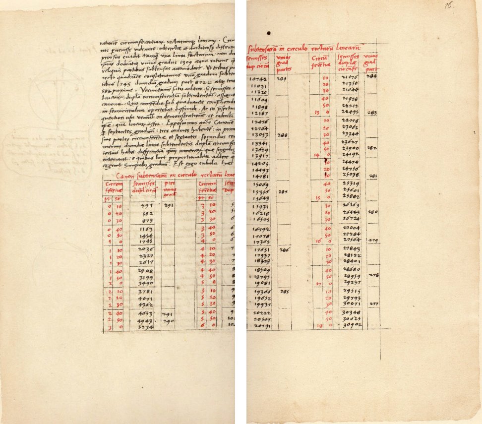 2. "To search for something – though it be mushrooms – or some pattern – is impossible, unless you look and try." Dmitri Mendeleev, Fundamentals of Chemistry, 1903. 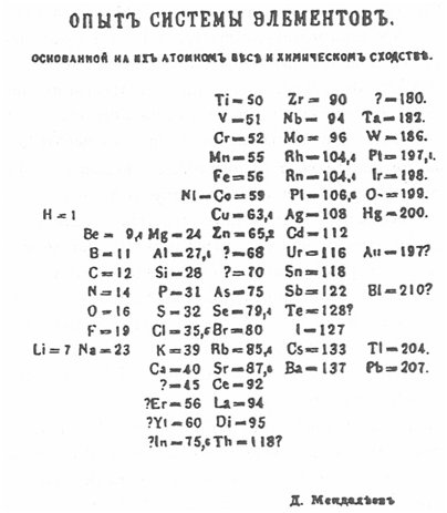 3. In a sense, we are Kepler-followers: "a mind to whom all ultimate reality, the essence of religion, of truth and beauty, was contained in the language of numbers." Arthur Koestler: The Sleepwalkers. Macmillan, 1959.  4. An intuitively accurate, but wrong model is Niels Bohr's model of the atom, where electrons are restricted to special energies with integer multiples of a unit energy.  5. Eine neue wissenschaftliche Wahrheit pflegt sich nicht in der Weise durchzusetzen, dass ihre Gegner überzeugt werden und sich als belehrt erklären, sondern vielmehr dadurch, dass die Gegner allmählich aussterben und dass die heranwachsende Generation von vornherein mit der Wahrheit vertraut gemacht worden ist. (Max Planck: Wissenschaftliche Selbstbiographie)  6. Actually, we have the inverse problem of climate change.  John von Neumann, his wife Klari, and their dog Inverse "Weather prediction is an initial value problem, climate prediction is a boundary condition problem" - he used to say. Applying the correct annual global mean boundary conditions – flux, cloud, albedo and energy budget stability constraints – on a 2 × CO2 atmosphere, GCMs might have the chance to provide us with some clue on the regional and seasonal distribution of the possible changes. 7. Did you know? Aristotle in his Meteorology lays down the basics of ocean Salinity and Flow: "Let us explain the nature of the sea and the reason why such a large mass of water is salt and the way in which it originally came to be. The
old writers who invented theogonies say that the sea has
springs, for they want earth and sea to have foundations and
roots
of their own. Presumably they thought that this view was
grander
and
more impressive as implying that our earth was an important
part of the universe. For they believed that the whole
world had been built up round our earth and for its sake, and
that the earth was the most important and primary part of it.
Others, wiser in human knowledge, give an account of its origin.
At first, they say, the earth was surrounded by moisture. Then
the
sun
began to dry it up, part of it evaporated and is the cause
of winds and the turnings back of the sun and the moon,
while the remainder forms the sea. So the sea is being dried up
and is growing less, and will end by being some day entirely
dried up. Others say that the sea is a kind of sweat exuded
by the
earth when the sun heats it, and that this explains its saltness:
for all sweat is salt. Others say that the saltness is due to
the
earth. Just as water strained through ashes becomes salt,
so the sea owes its saltness to the admixture of earth with
similar properties."
(...)
"The
whole of the Mediterranean does actually flow. The directionof
this flow is determined by the depth of the basins and by the
number of rivers. Maeotis flows into Pontus and Pontus into
the
Aegean.
After that the flow of the remaining seas is not so easy to
observe. The current of Maeotis and Pontus is due to the
number of rivers (more rivers flow into the Euxine and
Maeotis than into the whole Mediterranean with its much
larger basin), and to their own shallowness. For we find the sea
getting deeper and deeper. Pontus is deeper than Maeotis, the
Aegean than
Pontus, the Sicilian sea than the Aegean; the Sardinian and
Tyrrhenic being the deepest of all. (Outside the pillars of
Heracles the sea is shallow owing to the mud, but calm, for
it lies in a hollow.) We see, then, that just as single
rivers flow from mountains, so it is with the earth as a
whole: the greatest volume of water flows from the higher
regions
in the
north. Their alluvium makes the northern seas shallow,
while the outer seas are deeper. Some further evidence of
the height of the northern regions of the earth is afforded
by the view of many of the ancient meteorologists. They
believed that the sun did not pass below the earth, but round
its northern part, and that it was the height of this which
obscured
the sun and caused night."
(Which translation would you prefer?) 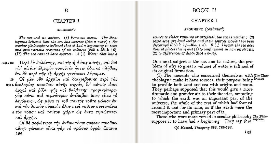 8. A map from 1935 shows the Mediterranean-Atlantic salt tongue this way: 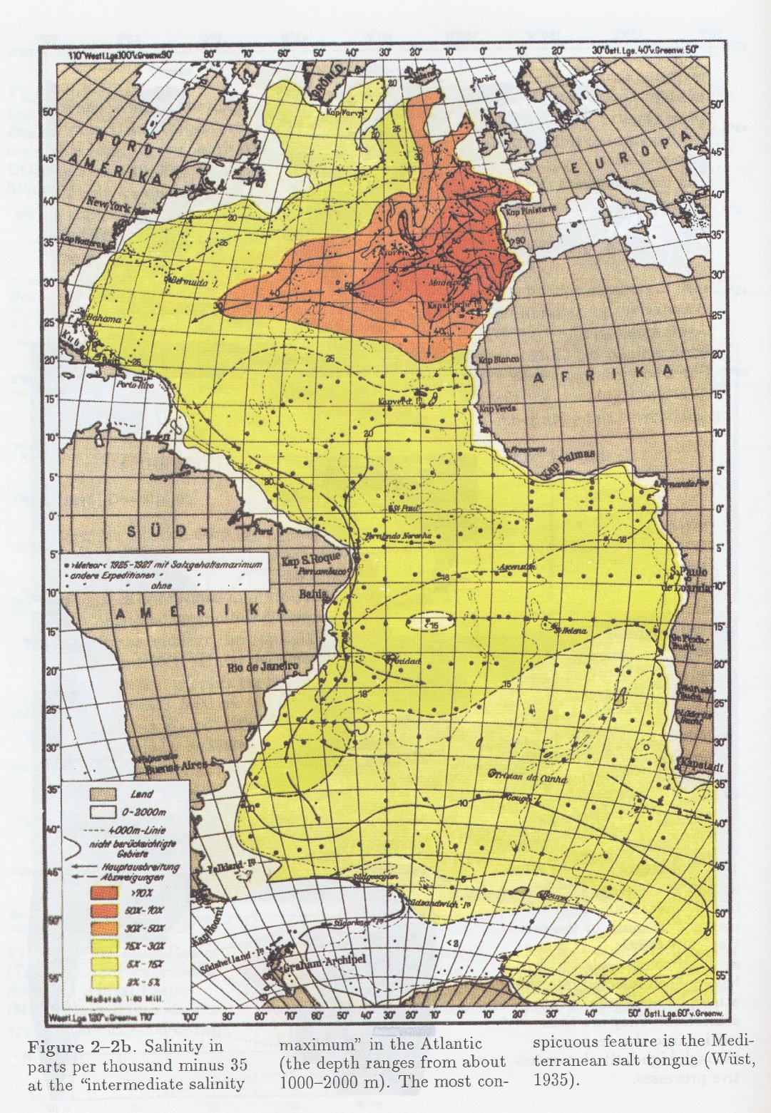 The slightest change in the Thermohalin Circulation might lead to change in the amount of upwelling coldwater from the abyss during the La Nina events, causing unpredictable variation in sea surface temperatures. 9. The best-known example for internal variability is the Broecker-conveyor:  |
|||||||||||||||||||||||||||||||||||||||||||||||||||||||||||||||||||||||||||||||||||||||||||||||||||||||||||||||||||||||||||||||||||||||||||||||||||||||||||||||||||||||||||||||||||||||||||||||||||||||||||||||||||||||||||||||||||||||||||||||||||||||
| Page created by: Miklós Zágoni Contact: info@globalenergybudget.com © Copyright information | |||||||||||||||||||||||||||||||||||||||||||||||||||||||||||||||||||||||||||||||||||||||||||||||||||||||||||||||||||||||||||||||||||||||||||||||||||||||||||||||||||||||||||||||||||||||||||||||||||||||||||||||||||||||||||||||||||||||||||||||||||||||