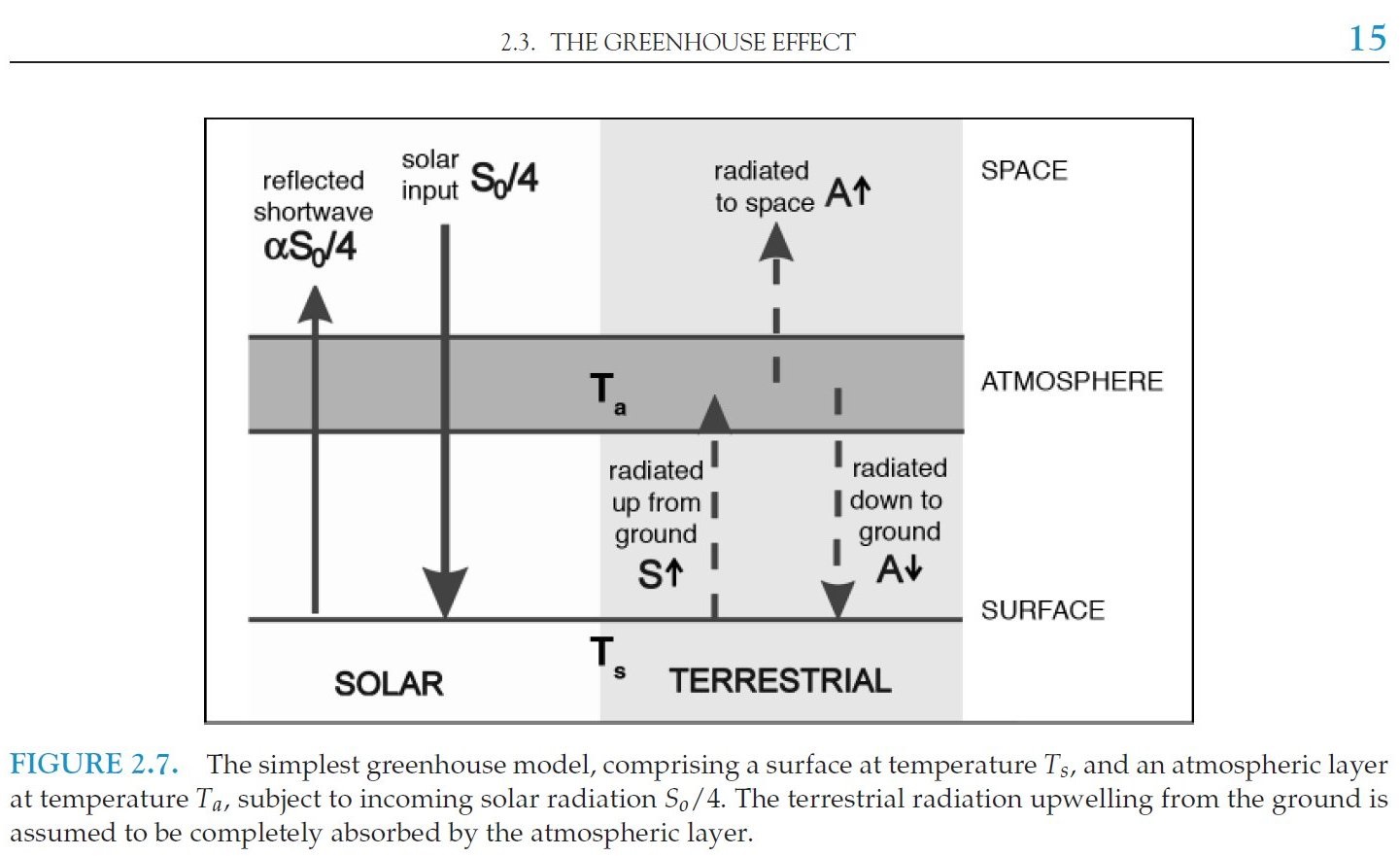
Marshall and Plumb (2007,
Fig. 2.7) show it this way:
Vardavas and Taylor's (Radiation and Climate, Oxford 2007) Fig.11.1 is essentially the same:
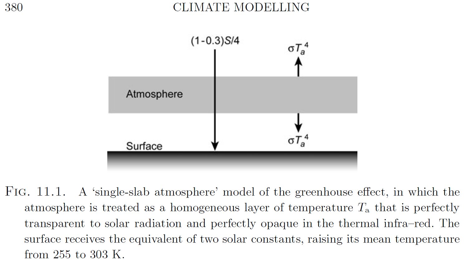

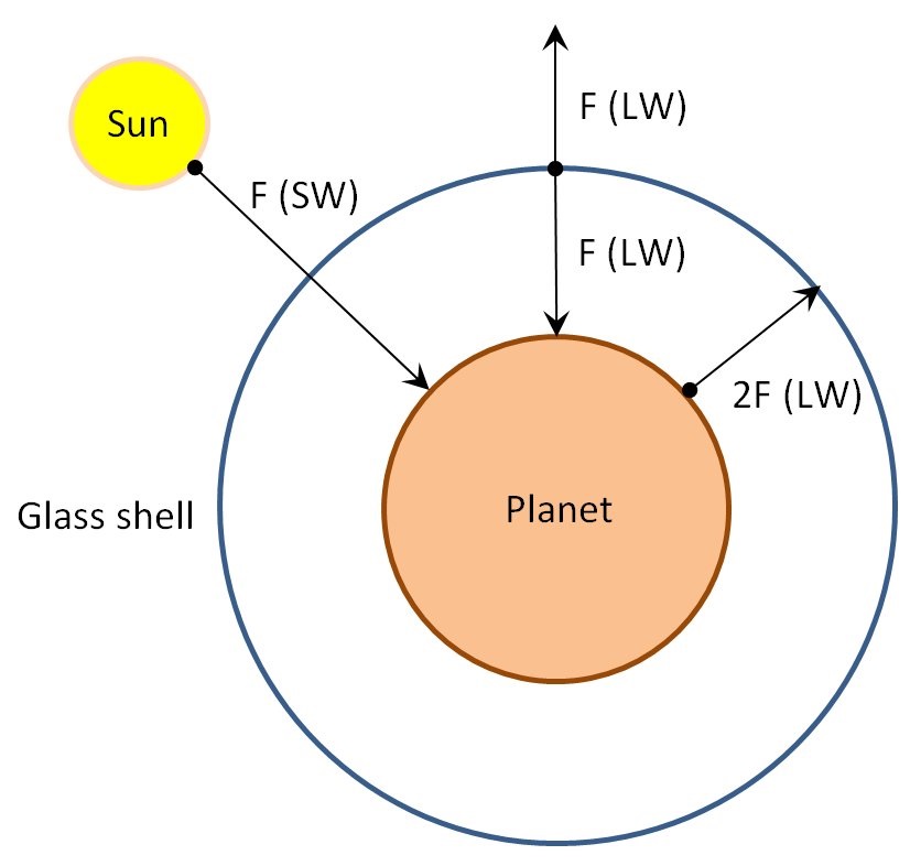
All of the figures above express the same relationship:
σTs4
= 2σTa4
S = 2A
That is, the surface receives (and emits) the equivalent of two solar 'constants' (the energy absorbed from the Sun).
We certainly do not think per se that this is true for the Earth.

A = 2A0 if m = 2
Here the referred Eq. (2.12) is the first term in Schwarzschild's (1906,
Eq. 11):
and Eq. (2.13) is the difference of the second and first terms in Schwarzschild's (1906, Eq. 11):
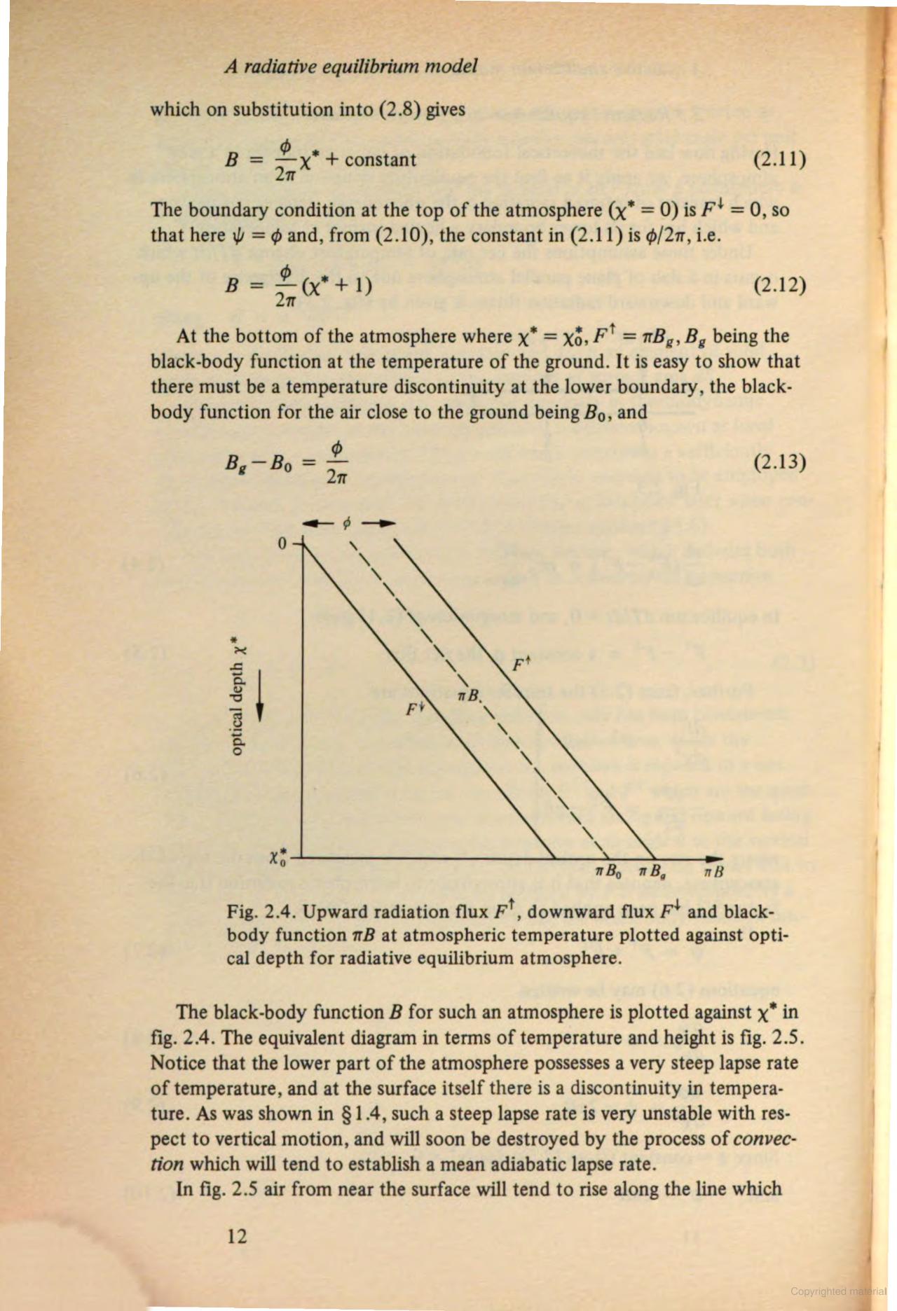
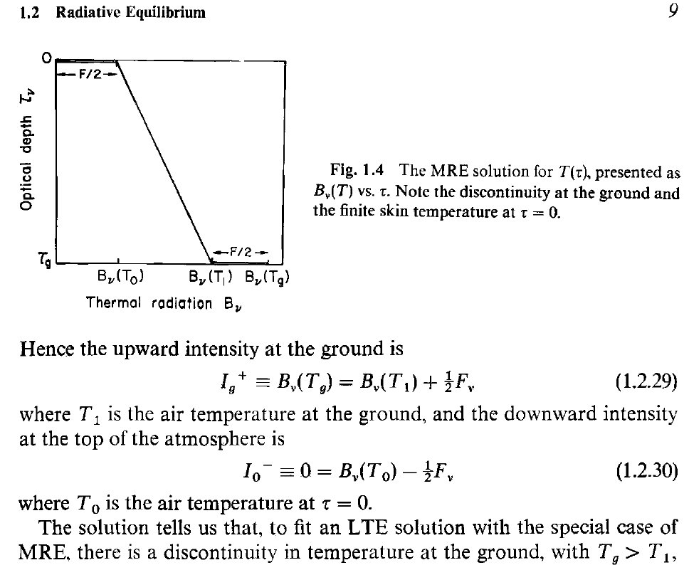
Hartmann (1994) shows the discontinuity:
Marshall and Plumb (2007) show the discontinuity:
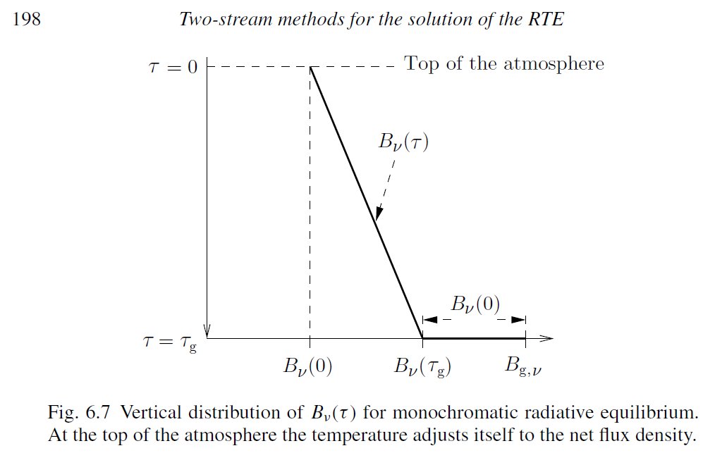
Zdunkowsky, Trautmann and Bott (Radiation in the Atmosphere, 2007) give the discontinuity and the first and second terms in Schw (1906, Eq. 11):
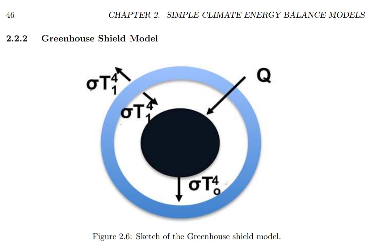
We have two equations here, both of them are τ-independent, that is, no reference to the gaseous composition of the atmosphere nor to the lapse rate, simply a consequence of the geometry:
S = 2A
That is, the surface receives (and emits) the equivalent of two solar 'constants' (the energy absorbed from the Sun).
We certainly do not think per se that this is true for the Earth.
Tyndall (1961), based on his earlier experiments, had no doubt that
as "the chief influence be exercised by the aqueous vapour, every
variation of this constituent must (sic) produce a change of climate."
Arrhenius (1896) already in the title of his famous essay ‘On the Influence of Carbonic Acid in the Air upon the Temperature of the Ground' is convinced about this relationship.
The dependence of absorption on the mass of the constituents (or, precisley, on their summarized "optische Masse", as Schwarzschild calls it) must be given by equations containing this m and the incoming solar radiation A0 (Schwarzschild 1906):
A being the upward beam at a layer (the emission of the layer, if that
layer is the lower boundary), and A0 the incoming solar energy (and outward
emission) at the upper boundary.
Now the equality above is the same
as the second term here, if m = 2 :
A = 2A0 if m = 2
Houghton (1977, The Physics
of Atmospheres) gives it as Eq. (2.15), when introducing the greenhouse
effect:
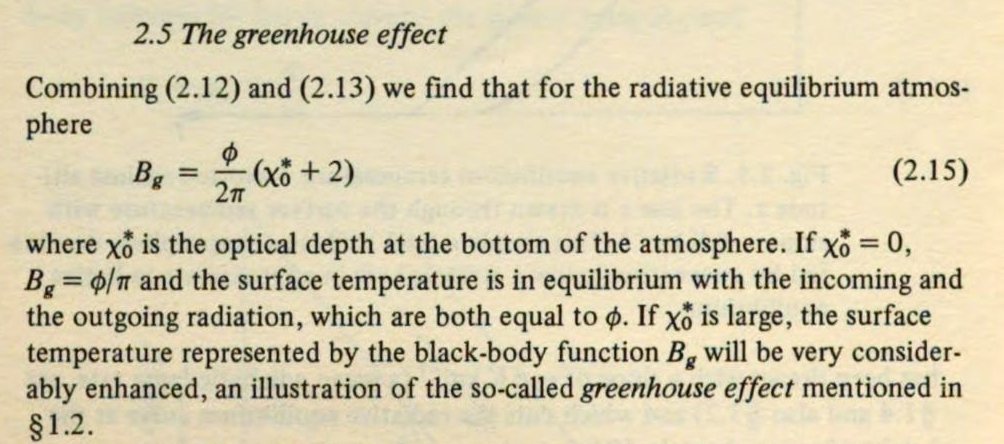
E = A0
(1 + m)/2
and Eq. (2.13) is the difference of the second and first terms in Schwarzschild's (1906, Eq. 11):
A – E = A0/2
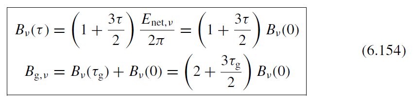
Chamberlain (Theory of Planetary Atmospheres, 1978) explains (using the more widespread τ instead of m for the oprical depth):
Hartmann (1994) shows the discontinuity:
Marshall and Plumb (2007) show the discontinuity:
Zdunkowsky, Trautmann and Bott (Radiation in the Atmosphere, 2007) give the discontinuity and the first and second terms in Schw (1906, Eq. 11):
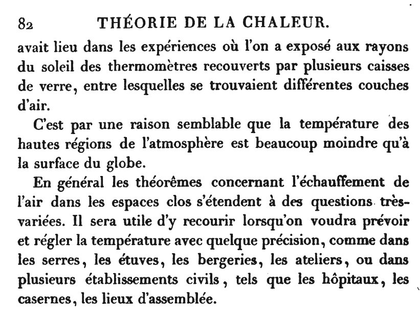
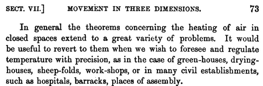
That is, after Tyndall and Arrhenius, there remained no doubt that the
atmospheric greenhouse effect is a direct function of the amount of
infrared absorbers. No one raised the question of whether the
original model of a glass plate, with its prescribed geometry and flux
ratios could be an alternative.
Here we do it, based on real Earth data.
Here we do it, based on real Earth data.
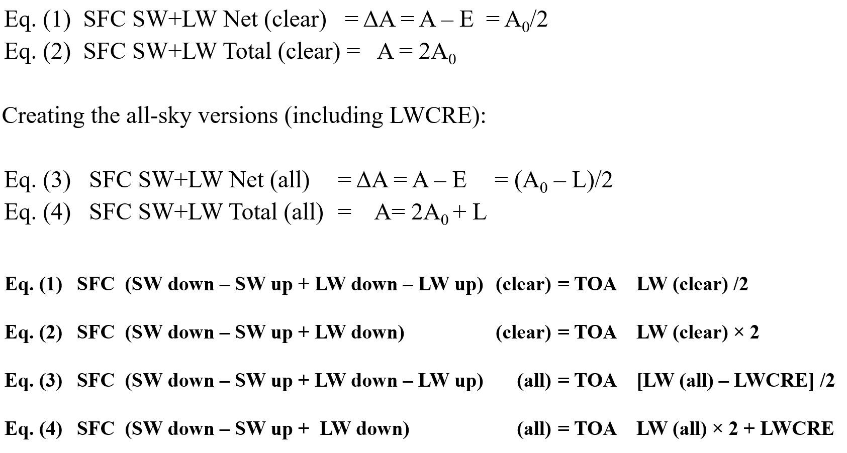
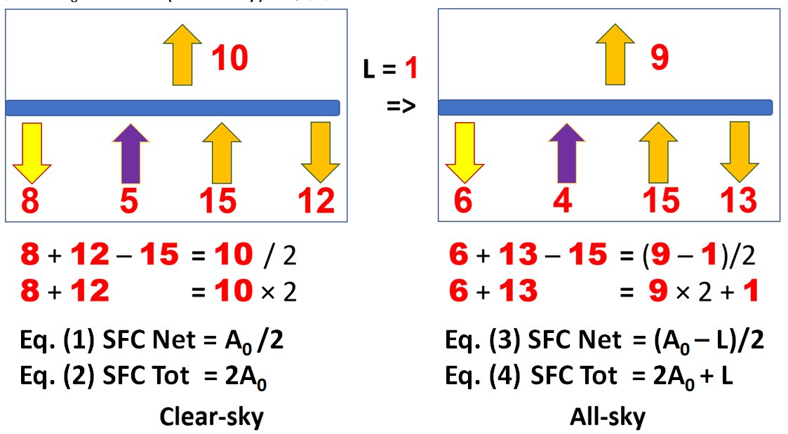
We have two equations here, both of them are τ-independent, that is, no reference to the gaseous composition of the atmosphere nor to the lapse rate, simply a consequence of the geometry:
Eq. (1) ΔA = A
– E = A0/2
Eq. (2) A = 2A0
The first equation describes the discontinuity at the surface in radiative equilibrium, equivalent to the net radiation at the surface and the corresponding non-radiative (convective) fluxes in readiative-convective equilibrium.
The second describes the total (SW + LW) energy absorption (= LW emission + turbulent fluxes) at the surface.
The corresponding ratios are:
ΔA : A0 : E : A = 1 : 2 : 3 : 4
The greenhouse effect is
G = E – A0,
and the normalized greenhouse factor is
g = G/E = (E – A0)/E = 1/3.
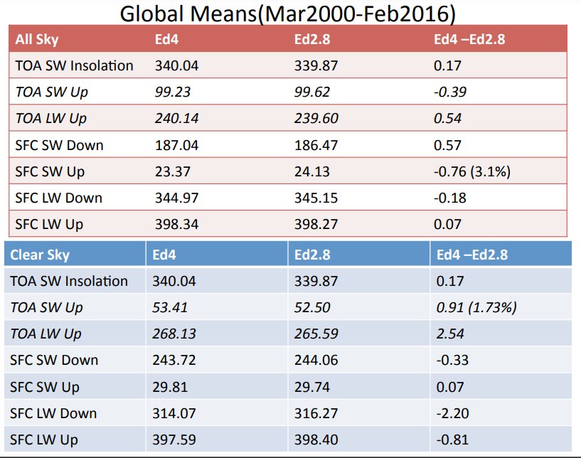
Let's check them on global mean Earth data.
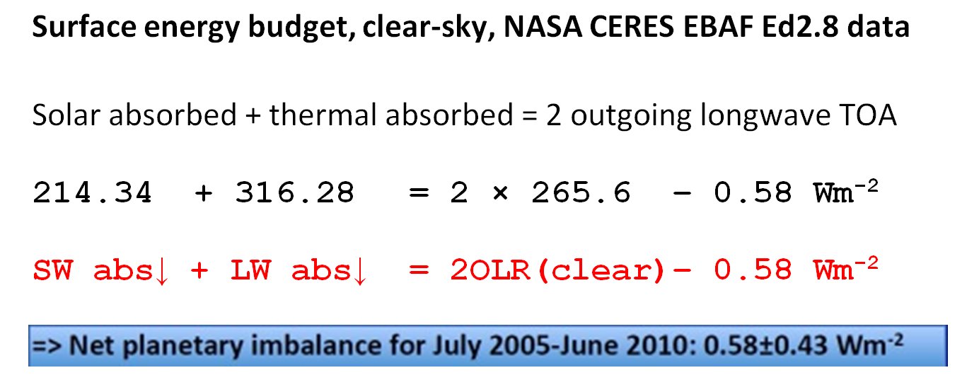
The data set available at the beginning of our research (2017) was CERES EBAF Ed2.8; with its global mean clear sky fluxes:
Eq. (2) A = 2A0
The first equation describes the discontinuity at the surface in radiative equilibrium, equivalent to the net radiation at the surface and the corresponding non-radiative (convective) fluxes in readiative-convective equilibrium.
The second describes the total (SW + LW) energy absorption (= LW emission + turbulent fluxes) at the surface.
The corresponding ratios are:
ΔA : A0 : E : A = 1 : 2 : 3 : 4
The greenhouse effect is
G = E – A0,
and the normalized greenhouse factor is
g = G/E = (E – A0)/E = 1/3.
Let's check them on global mean Earth data.
The data set available at the beginning of our research (2017) was CERES EBAF Ed2.8; with its global mean clear sky fluxes:
In this notation,
Eq. (1) Surface (SW down – SW up + LW down – LW up) = TOA LW up/2
244.06 – 29.74 + 316.27 – 398.40 = 265.59/2 – 0.605 Wm-2
The equation is valid with a difference of 0.605 Wm-2.
Eq. (2) Surface (SW down – SW up + LW down) = 2 × TOA LW up
244.06 – 29.74 + 316.27 = 2 × 265.59 – 0.59 Wm-2
The equation is valid with a difference of 0.59 Wm-2.
The accepted value of Earth's energy imbalance was 0.58 Wm-2 in that time.
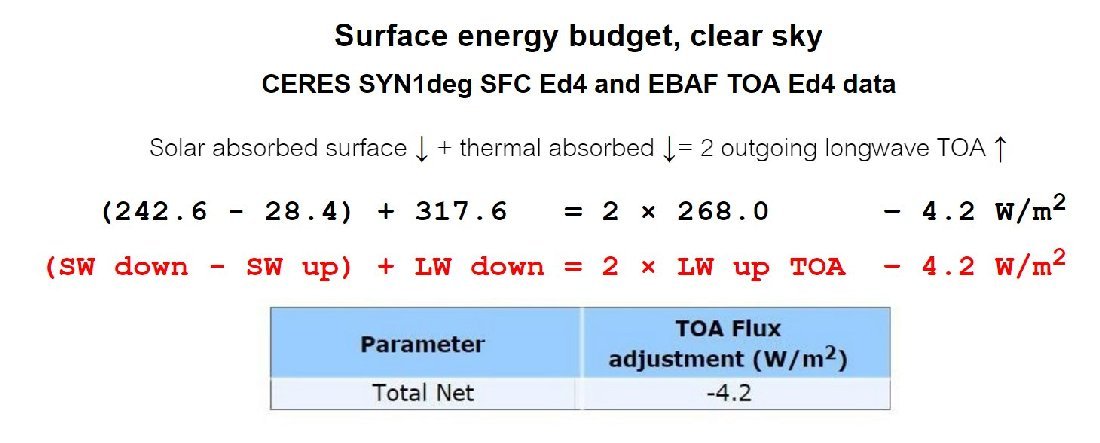
The precise validity of the glass-shell Eq. (2) on different CERES EBAF data products:
SYN1deg SFC Ed4 has a TOA flux adjustment of -4.2 Wm-2,
this is the accuracy of the equation:
EBAF Ed2.8 was adjusted to a net planetary imbalance of 0.58 Wm-2,
this is the accuracy of the equation:
Now the greenhouse effect:
G = Surface LW up – TOA LW up = 398.40 – 265.59 = 132. 81 Wm-2.
g = G/SFC LW up = 132.81 / 398.40 = 0.33336.
g(geometry) = 1/3.
We are not aware of any similar accuracy in climate science.
To our gratest surprise, Earth follows the simplest model of Fourier's greenhouse, and its basic structure is defined by that pane-of-glass geometry.
Greenhouse gases seem to play an executive rather than a decisive role: they have to implement and maintain what is required by the principles.
The best fit for the ratios:
ΔA : A0 : E : A = 1 : 2 : 3 : 4
is
ΔA : A0 : E : A = 1 : 2 : 3 : 4 = 5 : 10 : 15 : 20
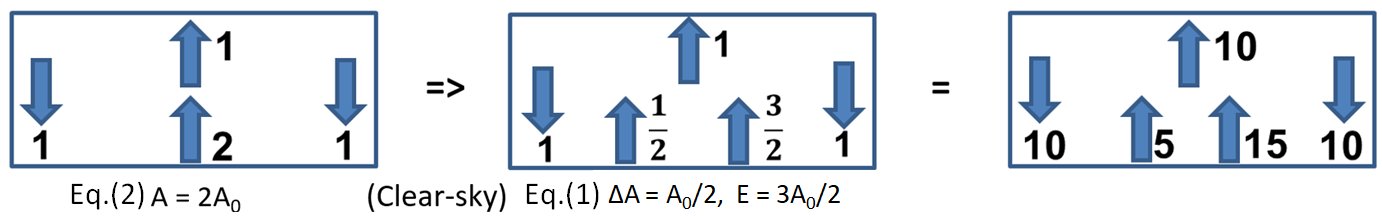
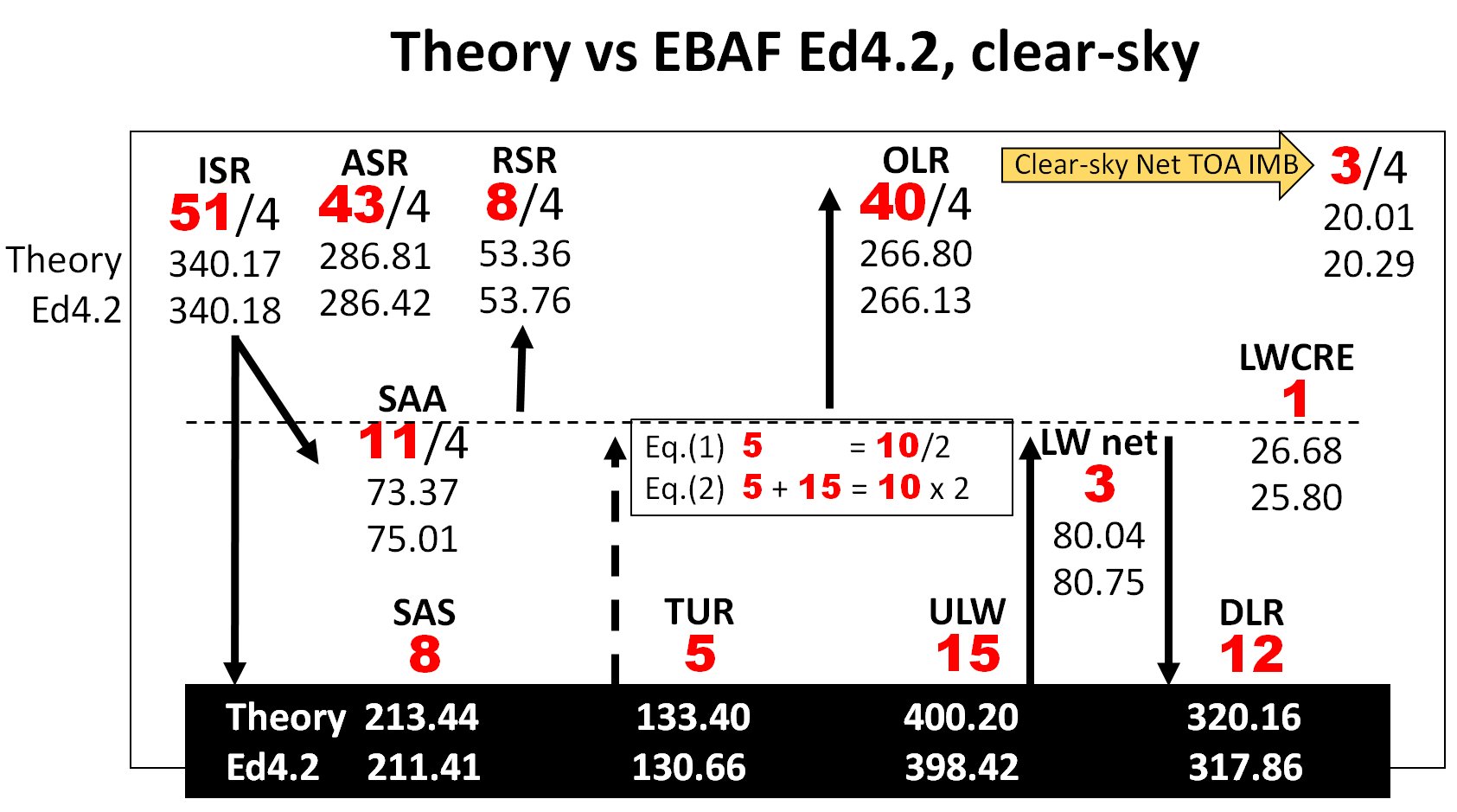
with 1 = 26.68 ± 0.01 Wm-2
With this, the theoretical geometric clear-sky greenhouse effect is
G = 5 = 133.40 Wm-2.
OLR = 10 = 266.80 Wm-2
ULW = 15 = 400.20 Wm-2
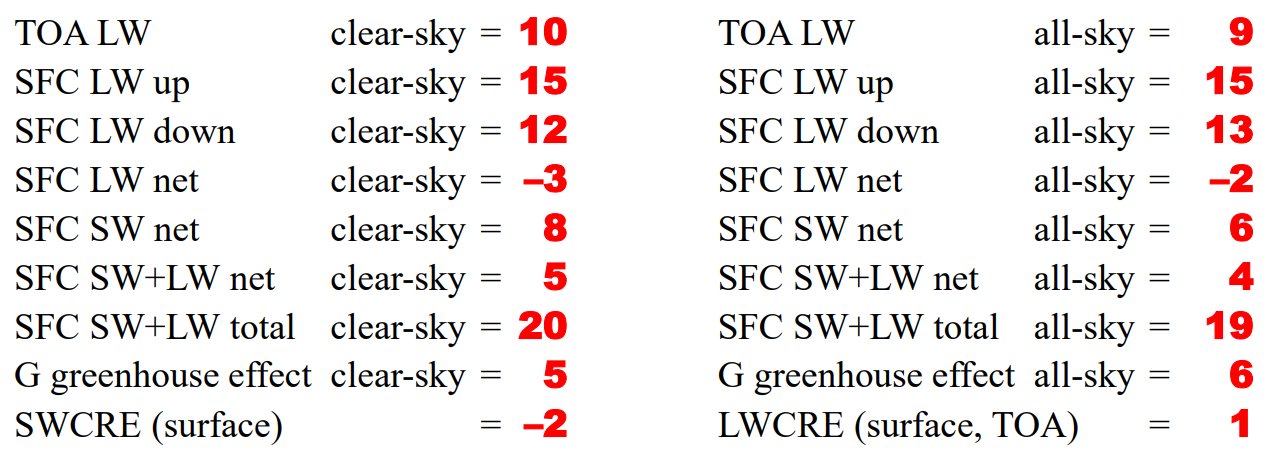
Observing that 1 = LWCRE,
g(clear-sky) = 1/3 = 5/15, g(LWCRE) = 1/15, we have g(all-sky) = 6/15 = 0.4,
and OLR(sll-sky) = 9 = 240.12 Wm-2.
g(all-sky) = 0.4 is confirmed by the IPCC WGI AR6 (2022) Fig. 7.2 with an unprecedented accuray:
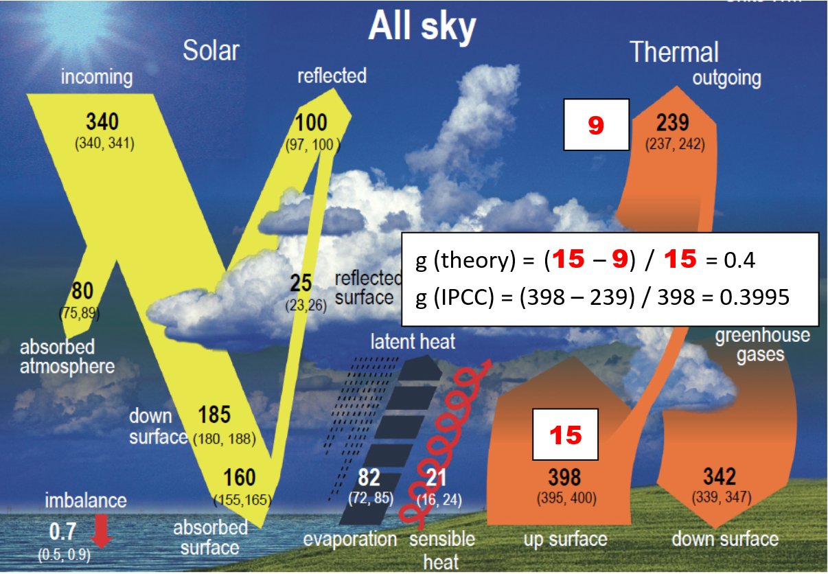
No deviation, no enhancement. Theory (glass-plate geometry) does not refer to GHGs.
Fine-tuning the model: All-sky equations:
Verifying the all-sky equations on CERES EBAF Ed4.1 (April 2000 - March 2022) data:
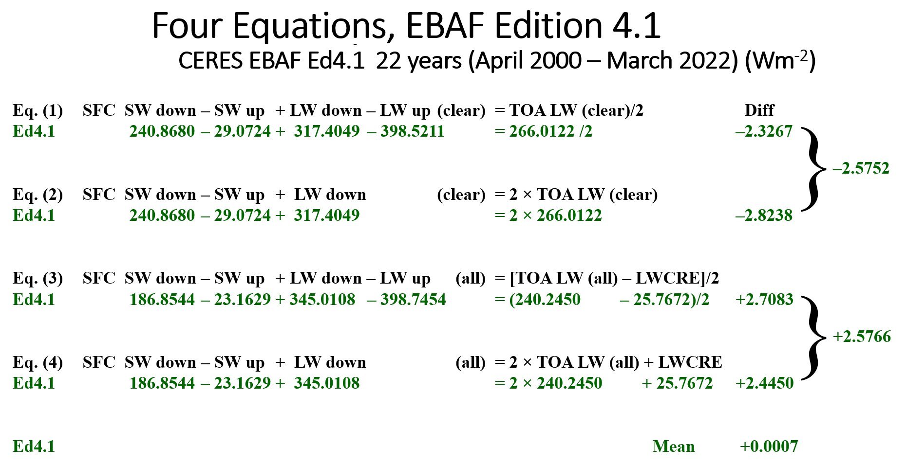
Individual deviation is less than ±3 Wm-2; the four equations together have a mean bias of 0.0007 Wm-2.
The fine-tuned "Fourier" glass-shield geometry:
The complete extended geometric "Fourier" N-system:
TOA extension from geometric deduction vs EBAF:
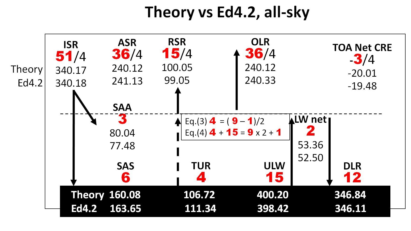
Eq. (3) and (4), all-sky versions of the original clear-sky net and total,
are confirmed by the most recent GEWEX (2023, BAMS) research
with the exemplary accuracy of 0.1 Wm-2:
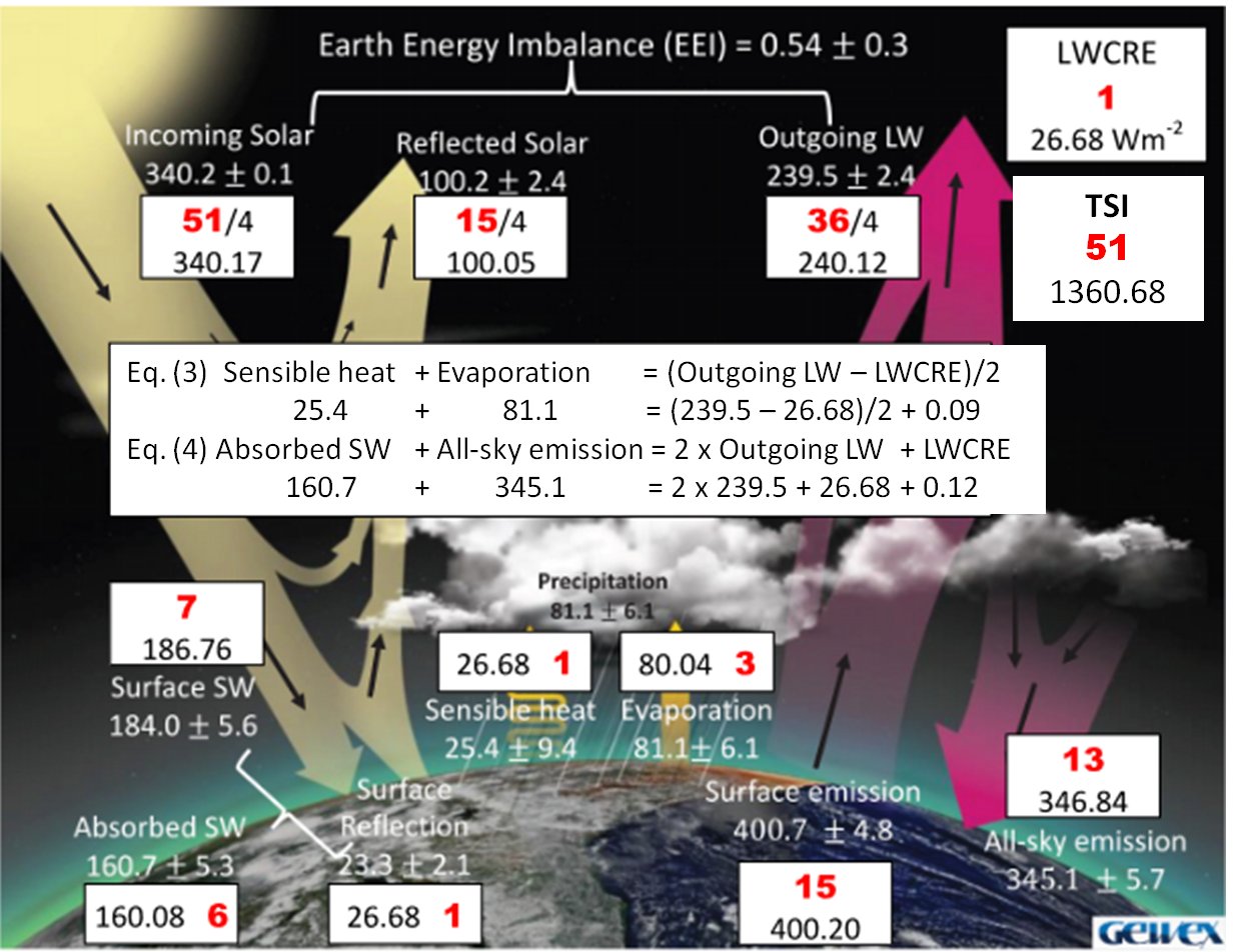
Details of the geometric deduction (taking into account that the Earth's atmosphere is not completely SW-transparent nor perfectly LW-opaque) were given above.
Window, and the interplay of clear and cloudy regions to create an effectively IR-opaque (glass-shell-like) atmosphere by the help of LWCRE will be discussed below.
Let us assume, we have a wonderful instrument measuring the all-sky global mean Atmospheric LW Cooling as 186.76 Wm-2, or the clear-sky surface net LW as 80.04 Wm-2. We know from the integer system that the former is 7 units, the latter is 3 units; or we may have any of the components. From these, we would know for sure that 1 unit is 26.68 Wm-2.
Let us allow a ± 0.01 Wm-2 uncertainty.
Then what we have to do is to fit TSI to the UNIT:
TSI = 51 = 51 × 26.68 ± 0.01 = 1360.68 ± 0.5 Wm-2 in spherical weighting
TSI = 51 = 51 × 26.68 × (4.0034/4) = 1361.84 ± 0.5 Wm-2 in geodetic weighting.
Only from having accurate measurements of ANY of the internal fluxes, either all-sky or clear-sky, SW or LW, we can tell very accurate how much energy MUST arrive from the Sun to maintain that measured flux component.
To sum-up here:
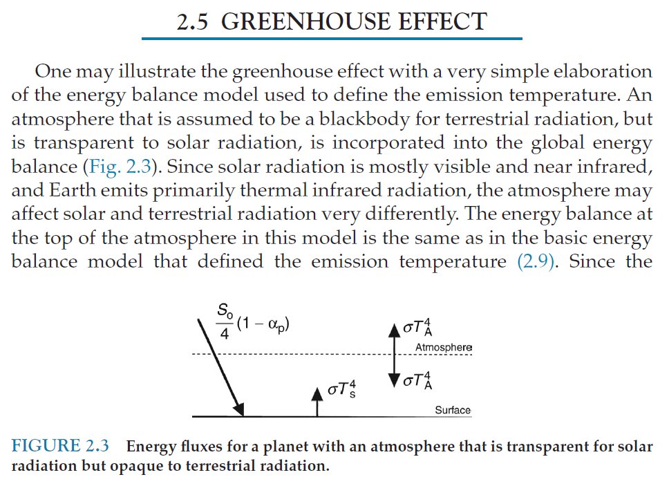
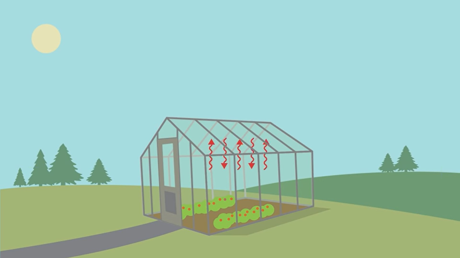
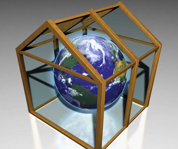
Imagine the atmosphere is condensed into a single layer, to mimick the pane of glass model of Fourier.
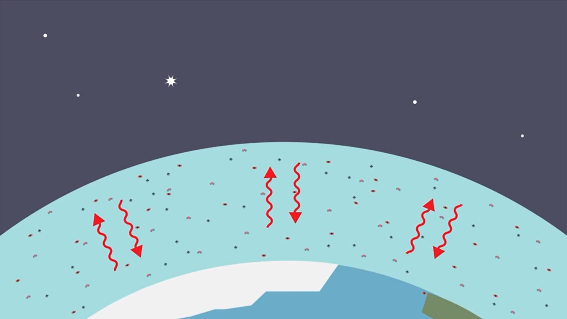
In our realistic case, the layer consists of three horizontal regions:
- an IR-opaque region from an effective cloud area fraction (9/15 = 0.6),
- an IR-opaque clear-sky region by GHGs (5/15 = 1/3),
- and a transprent clear-sky region (WIN = 1/15).
This setup, with the corresponding ruling principles and the equations describing them,
accurately reproduce the Earth's annual global mean energy flow system.
See Science implications.
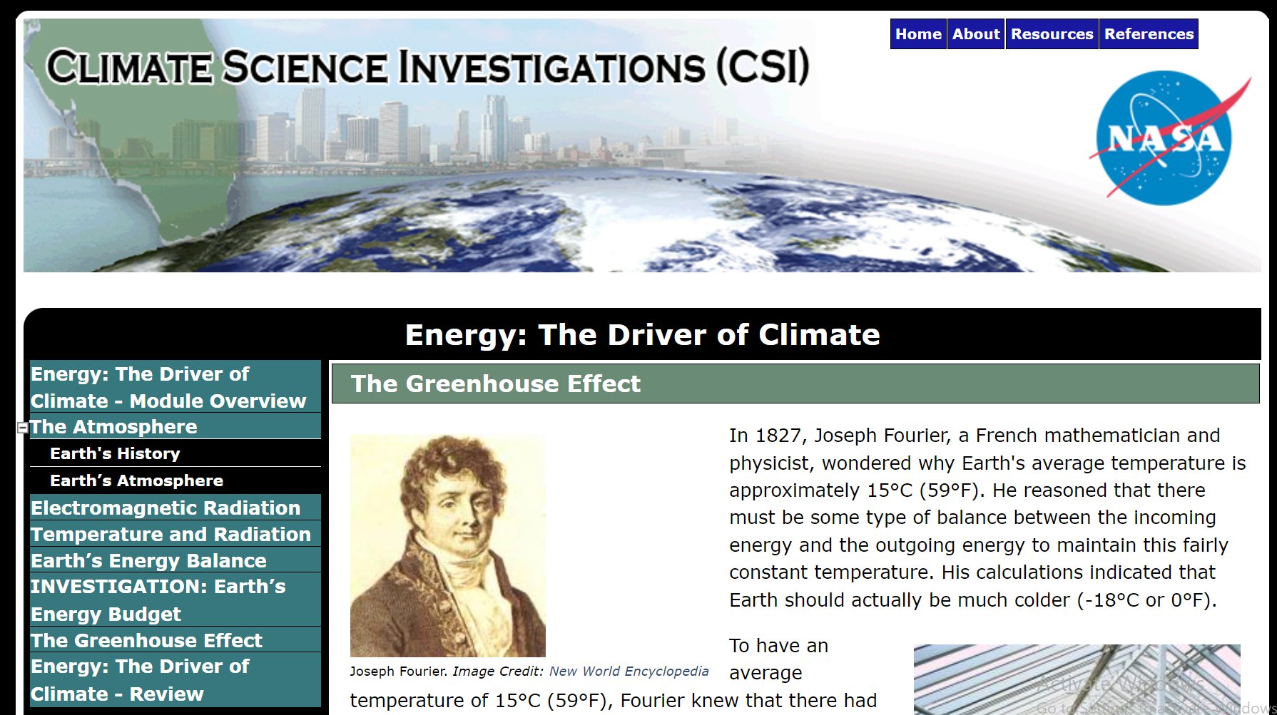
NASA got it right:


Perfect.
It seems the glasshouse model really works.
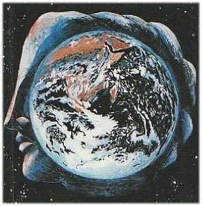
We have a wonderfully shielded Earth.

We only wish Gaia knows what She's doing.
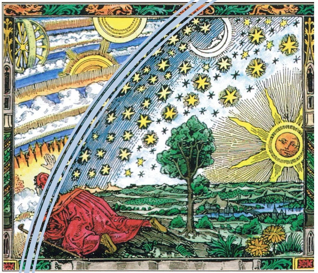
It would be great to have a look behind the shield to see the wheels.
Go to the next page "Trenberth's greenhouse geometry" or jump back to the main "index" page.
Eq. (1) Surface (SW down – SW up + LW down – LW up) = TOA LW up/2
244.06 – 29.74 + 316.27 – 398.40 = 265.59/2 – 0.605 Wm-2
The equation is valid with a difference of 0.605 Wm-2.
Eq. (2) Surface (SW down – SW up + LW down) = 2 × TOA LW up
244.06 – 29.74 + 316.27 = 2 × 265.59 – 0.59 Wm-2
The equation is valid with a difference of 0.59 Wm-2.
The accepted value of Earth's energy imbalance was 0.58 Wm-2 in that time.
The precise validity of the glass-shell Eq. (2) on different CERES EBAF data products:
SYN1deg SFC Ed4 has a TOA flux adjustment of -4.2 Wm-2,
this is the accuracy of the equation:
EBAF Ed2.8 was adjusted to a net planetary imbalance of 0.58 Wm-2,
this is the accuracy of the equation:
Now the greenhouse effect:
G = Surface LW up – TOA LW up = 398.40 – 265.59 = 132. 81 Wm-2.
g = G/SFC LW up = 132.81 / 398.40 = 0.33336.
g(geometry) = 1/3.
We are not aware of any similar accuracy in climate science.
To our gratest surprise, Earth follows the simplest model of Fourier's greenhouse, and its basic structure is defined by that pane-of-glass geometry.
Greenhouse gases seem to play an executive rather than a decisive role: they have to implement and maintain what is required by the principles.
The best fit for the ratios:
ΔA : A0 : E : A = 1 : 2 : 3 : 4
is
ΔA : A0 : E : A = 1 : 2 : 3 : 4 = 5 : 10 : 15 : 20
with 1 = 26.68 ± 0.01 Wm-2
With this, the theoretical geometric clear-sky greenhouse effect is
G = 5 = 133.40 Wm-2.
OLR = 10 = 266.80 Wm-2
ULW = 15 = 400.20 Wm-2
Observing that 1 = LWCRE,
g(clear-sky) = 1/3 = 5/15, g(LWCRE) = 1/15, we have g(all-sky) = 6/15 = 0.4,
and OLR(sll-sky) = 9 = 240.12 Wm-2.
g(all-sky) = 0.4 is confirmed by the IPCC WGI AR6 (2022) Fig. 7.2 with an unprecedented accuray:
No deviation, no enhancement. Theory (glass-plate geometry) does not refer to GHGs.
Fine-tuning the model: All-sky equations:
Verifying the all-sky equations on CERES EBAF Ed4.1 (April 2000 - March 2022) data:
Individual deviation is less than ±3 Wm-2; the four equations together have a mean bias of 0.0007 Wm-2.
The fine-tuned "Fourier" glass-shield geometry:
The complete extended geometric "Fourier" N-system:
TOA extension from geometric deduction vs EBAF:
Eq. (3) and (4), all-sky versions of the original clear-sky net and total,
are confirmed by the most recent GEWEX (2023, BAMS) research
with the exemplary accuracy of 0.1 Wm-2:
Details of the geometric deduction (taking into account that the Earth's atmosphere is not completely SW-transparent nor perfectly LW-opaque) were given above.
Window, and the interplay of clear and cloudy regions to create an effectively IR-opaque (glass-shell-like) atmosphere by the help of LWCRE will be discussed below.
Let us assume, we have a wonderful instrument measuring the all-sky global mean Atmospheric LW Cooling as 186.76 Wm-2, or the clear-sky surface net LW as 80.04 Wm-2. We know from the integer system that the former is 7 units, the latter is 3 units; or we may have any of the components. From these, we would know for sure that 1 unit is 26.68 Wm-2.
Let us allow a ± 0.01 Wm-2 uncertainty.
Then what we have to do is to fit TSI to the UNIT:
TSI = 51 = 51 × 26.68 ± 0.01 = 1360.68 ± 0.5 Wm-2 in spherical weighting
TSI = 51 = 51 × 26.68 × (4.0034/4) = 1361.84 ± 0.5 Wm-2 in geodetic weighting.
Only from having accurate measurements of ANY of the internal fluxes, either all-sky or clear-sky, SW or LW, we can tell very accurate how much energy MUST arrive from the Sun to maintain that measured flux component.
To sum-up here:
Imagine the atmosphere is condensed into a single layer, to mimick the pane of glass model of Fourier.
In our realistic case, the layer consists of three horizontal regions:
- an IR-opaque region from an effective cloud area fraction (9/15 = 0.6),
- an IR-opaque clear-sky region by GHGs (5/15 = 1/3),
- and a transprent clear-sky region (WIN = 1/15).
This setup, with the corresponding ruling principles and the equations describing them,
accurately reproduce the Earth's annual global mean energy flow system.
See Science implications.
NASA got it right:
Perfect.
It seems the glasshouse model really works.
We have a wonderfully shielded Earth.
We only wish Gaia knows what She's doing.
It would be great to have a look behind the shield to see the wheels.
Go to the next page "Trenberth's greenhouse geometry" or jump back to the main "index" page.