Easy
We are going to present four types of patterns:
.
I.
Integer relationships.
Look at the following numbers:
106
238.5
345
398
.
26.5
.
What can you see?
The first four numbers are integer multiples of the fifth, with 0.0 or 0.5 difference:
:
106 = 4 × 26.5 (+ 0.0)
238.5 = 9 × 26.5 (+ 0.0)
345 = 13 × 26.5 (+ 0.5)
398 = 15 × 26.5 (+ 0.5)
These are numerical values of five different energy flows in the global energy budget, and are measured in watts per square metre, W/m2.
One paper gave the non-radiative (turbulent) fluxes, which is the sum of the Latent Heat (LH) and Sensible Heat (SH) release from the surface, as LH + SH = 106 W/m2.
Another paper presented the Outgoing Longwave Radiation (OLR) of the Earth-atmosphere system, based on the most recent satellite observations; this was OLR = 238.5 W/m2.
Again another paper presented the downward emission from the atmosphere to the surface, called also “back-radiation”, its most common name is Downward Longwave Radiation; this was DLR = 345 W/m2.
The same paper presented the annual mean black-body (Planck) radiation of the Earth’s surface, called Upward Long-Wave radiation; this was ULW = 398 W/m2.
And the first paper referred here mentions also a quantity measured by NASA CERES (Clouds and the Earth’s Radiant Energy System) satellites, which is the numerical value of a substantial climate parameter called Long Wave Cloud Radiative Effect, LWCRE = 26.5 W/m2.
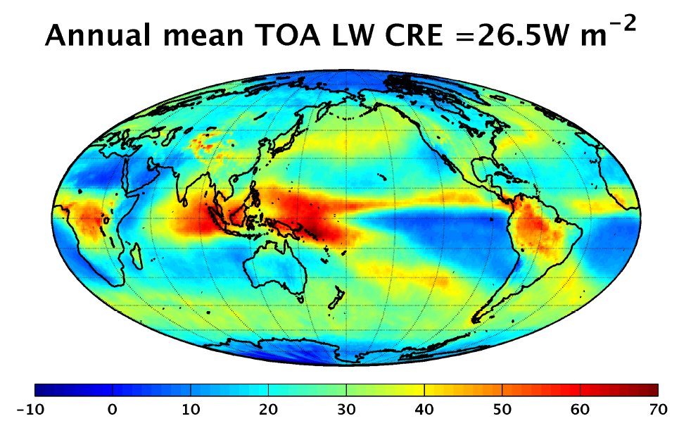
(Observed top-of-atmosphere Longwave Cloud Radiative Effect)
*
Our first result is a simple recognition: the above-referred, published, observed and modeled values of certain fundamental energy flows in the climate system are integer multiples of another.
It is important to note that some of the above-cited publications give also uncertainty estimates (error bounds) to their values: ± 1σ range. About the latter, Stevens and Schwartz (2012) say in the legend of their global energy budget diagram: “the authors assign a roughly 68 % likelihood that the actual values fall within the stated range”.
Now look at the following numbers (1σ):
± 7
± 2
± 7
± 3
± 5.
These are the said 1σ ranges of the above-given observed values of the fluxes of LH + SH, OLR, DLR, ULW and LWCRE, respectively.
And in the following four numbers (Δ):
0.0
0.0
+ 0.5
+ 0.5
we repeated the Δ differences of the observed mean values of the fluxes from their integer multiple of LWCRE.
As it can be seen, the Δ differences are much smaller that the attached 1σ uncertainty ranges.
This peculiar feature is repeated when we examined the other observable energy flow components of the global energy budget. We found that they fit into the same structure, and their best values can also be written as I × LWCRE, where I is an integer between 1 and 15 and LWCRE is as given above, well within the difference of the observed error.
Actually, we were able to reach a better fit for the recently published observational values of all flux elements when utilized LWCRE = 26.6 W/m2. Interestingly, this LWCRE value is presented in an independent NATURE Geoscience energy budget publication in 2012.
So we described the observed longwave and the shortwave radiations, and also the non-radiative flux elements – Sensible Heat (SH) and Latent Heat (LH) – in this way:
where F0 is generated as
and ΔF for each flux element was much smaller than the typical 1σ observational uncertainty.
There are also non-observable flux components in the global energy budget, like Longwave Atmospheric Absorption (LAA), or the surface upward longwave radiation that escapes through the infrared “atmospheric window”, called Surface Transmitted Irradiance (STI).
Importantly, there are published accurate computational results in the literature for these components — and they fit also into the integer pattern very precisely.
This characteristic of the fluxes is so surprising that we had to look after some theoretical explanation; and, based on other observations, we have found a quite natural one. But let us emphasize: the validity of the found relationships does not depend on the validity of the proposed physical interpretation.
.
II.
Energy balance constraints
(+ a conceptual framework)
The second basket of our results is a theoretical framework for this peculiar behaviour of fluxes.
We start with an observation again: the published value of the so-called “atmospheric window” radiation (STI) is about one-fifteenth of the surface upward radiation. That is, the other part (14/15) of ULW is absorbed by the atmosphere. Our atmosphere is almost-opaque to the terrestrial radiation: the absorption cross-section of the infrared-active gases (the so-called greenhouse gases: water vapour, carbon dioxide, methane, ozone and some others) cover almost the entire spectrum of the longwave radiation emitted by the Earth’s surface at an annual global mean surface temperature of Ts = 288 °Kelvin (15 °Celsius).
We then examined the ‘end-of-the-road’ model, when our partially-transparent atmosphere became entirely opaque for the terrestrial longwave radiation.
This model has a simple geometry (a planet being closed into a glass shell), and has a very easy relationship for its surface energy balance:
Energy (surface, LW-opaque atmospheric model) = ULW = 2OLR.
We then checked this relationship on the clear-sky (cloudless) part of the Earth’s atmosphere. The data are given by NASA CERES satellite missions. And, to our greatest surprise, the energy balance equation for the cloudless part of the Earth looks the same as in the closed-shell model
Energy (surface, Earth, clear-sky) = ULW + SH + LH = 2OLR(clear).
Further, in the all-sky case (this term stands for the average cloudy + cloudless conditions), the data show that the structure is the same, but there is some missing energy from the surface – which we identified as quantitatively equal to the loss in the “atmospheric window”, i.e., as surface transmitted irradiance in the all-sky mean.
Energy (surface, Earth, all-sky) = ULW + SH + LH = 2OLR(clear) — STI(all).
Another interesting recognition: this value is the same as (at least, statistically indistinguishable from) the above-referred LWCRE, which is the heating (blanketing) effect of the cloud cover.
So the idea came: from an energetic point of view, isn’t the role of clouds to fill the gap? To close the atmospheric window? This would explain the numerical validity of the closed-model analogy: what is lost (from a surface perspective) in the window, is gained back by the clouds:
Energy (surface, Earth, all-sky) = ULW + SH + LH = 2OLR(all) + LWCRE.
This idea would make understandable why the specific ‘closed-model’ energy budget relationships work well in Earth.

But the overall importance of this model is that it explains in one coherent theoretical framework BOTH of the two particular features TOGETHER: the integer pattern of the fluxes (which is exactly the behaviour we expect from waves propagating in a box) AND the constraint relationships in the surface energy budget (which is exactly the behaviour we expect from the closed-model geometry).
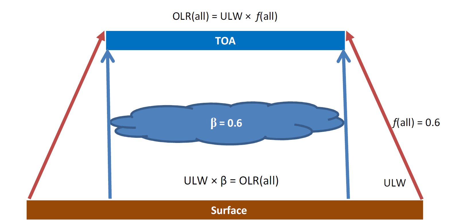
This model leads to a relationship between the annual global mean surface upward longwave radiation, ULW, and all-sky outgoing longwave radiation at the top of atmosphere, OLR(all) as
OLR(all) = 3/5 ULW.
It is termed also planetary emissivity:
- "the ratio between the radiation to space and the radiation from the surface of the Earth", Bengtsson 2012: Foreword to the special issue on Observing and Modeling Earth's Energy Flows);
- called also normalized longwave TOA (top of the atmosphere) flux; Inamdar and Ramanathan 1997: On monitoring the atmospheric greenhouse effect from space);
- or transfer function, defined as LW (up, TOA) / LW (up, surface) = LW Trans = L↑t / L↑s by Rossow and Zhang 1995: Calculation of surface and top-of-atmosphere radiative fluxes from physical quantities.
It's quantity is:
ep = OLR(all) / ULW = f(all) = 0.6.
Let us check it on the above data:
OLR(all) = 238.5 W/m2, ULW = 398 W/m2, hence f(all) = 0.6,
far within to the observation error.
[ CERES EBAF Ed2.8: f(all) = 0.6017 ]
.
III.
Cloud area fraction.
The cooperation of the clear and the cloudy parts of the atmosphere requires global (planetary level) energetic interactions, and the cloud area fraction is a substantial parameter here.
It is measured again by the NASA CERES satellite missions, and its observed value, 60.5% as a mean for the past decade, connects the total IR-opaque single-layer cloud area fraction β to the planetary emissivity at a value of
ep = OLR(all) / ULW = f(all) = β = 0.6.
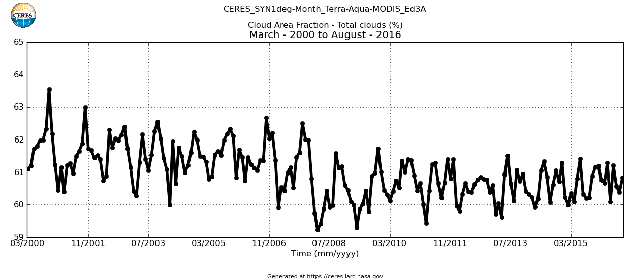
(Observed cloud area fraction)
*
β × ULW = OLR(all).
The importance of a constrained cloud area fraction is evident also from the point of view of shortwave reflectivity.
IV.
Albedo.
Acknowledging the different types of interaction between light and matter in the shortwave and in the longwave parts of the spectrum, and hence accepting the usefulness of the distinction between solar and terrestrial radiations (manifested also in the different boundary conditions for SW and LW at the top of the atmosphere, where LWdown = 0), it should still be noted that from a general energetic point of view, both of them are part of the same physical phenomenon of electromagnetic radiation.
Hence the ‘box model’, with the conditions of transparent in the SW and opaque in the LW, might be of some usefulness for the solar radiation as well.
From this, with only a preliminary, inconclusive recognition, we can realize that the 'box' (including the cloud surface and the land-ocean Earth surface) behaves in a way that a preferred value for the planetary albedo is formed.
Incoming Solar
Radiation
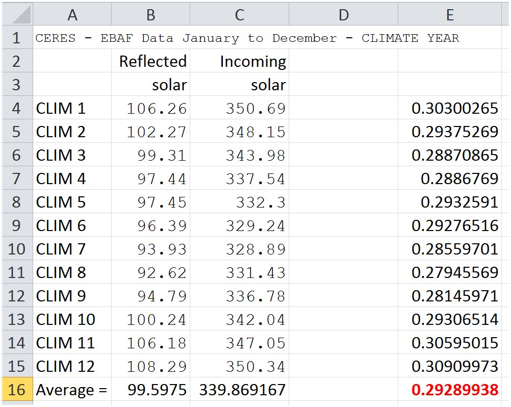
is accurately measured by satellites as ISR = 339.87 ±
0.2
W/m2, and
Reflected Solar Radiation as RSR = 99.6 ± 1 W/m2.
Their difference is
Absorbed Solar Radiation in the system is ISR – RSR = ASR = 240.3 W/m2,
hence the ratio of the reflected flux to the incoming flux, which is the planetary albedo, is then:
α = RSR / ISR = 99.6 / 339.87 = 1 – sin 45° = 1 – √2/2 = 0.29289.
The same paper observes a "surprising", "dramatic" hemispheric symmetry: “the Northern and Southern Hemispheres reflect the same amount of sunlight within ~ 0.2 Wm/2", contrary to entirely different ground conditions.
Adding to these, the paper finds that "The albedo of Earth appears to be highly buffered on hemispheric and global scales as highlighted by both the hemispheric symmetry and a remarkably small interannual variability of reflected solar flux (~0.2% of the annual mean flux)."
The detailed cooperation
- between the hemispheres;
- between the clear and cloudy reflectivity;
- between the surface and atmospheric absorptions and reflections;
- within the subsequent years
evidently requires strict planetary-level energetic regulations — or a definite geometry.