SURFACE ENERGY BUDGET
CERES EBAF-Surface_Ed2.8 data
Kato, S., N. G. Loeb, F. G. Rose, D. R. Doelling, D. A. Rutan, T. E. Caldwell, L. Yu, and R. A. Weller, 2013: Surface irradiances consistent with CERES-derived top-of-atmosphere shortwave and longwave irradiances. J. Climate, 26, 2719-2740, doi:10.1175/JCLI-D-12-00436.1.
Data were obtained from the NASA Langley Research Center CERES ordering tool at http://ceres.larc.nasa.gov/.
INTRODUCTION
In this webpage we are going to analyze NASA CERES (Clouds and the Earth’s Radiant Energy System) EBAF (Energy Balanced and Filled) data, in order to establish best estimates for the Earth’s surface energy budget. We use annual global mean data for time period 2001-2015; monthly climate year data; and 15-year averages as presented in the CERES EBAF TOA and Surface Data Quality Summaries. The current edition is Ed2.8; Ed4.0 is coming soon; we also use data from the available Ed4.0 prototype edition.
The surface energy budget has the following components. Energy income: absorbed solar radiation (downward less reflected surface solar flux) plus longwave emission from the atmosphere to the surface (Downward Longwave Radiation, DLR, termed also back radiation). Energy out: Upward LongWave (ULW) emission (surface Planck-radiation) plus turbulent fluxes: conduction, convection (Sensible Heat, SH) and evaporation (Latent Heat, LH). Under equilibrium, the in and out fluxes are equal; recently a certain imbalance is observed in a magnitude of about 0.6 W/m2.
The measured TOA (top-of-the-atmosphere) fluxes are the followings: Incoming Solar Radiation (ISR), Reflected Solar Radiation (RSR; albedo = RSR/ISR); their difference is Absorbed Solar Radiation (ASR) [it has two components: Solar Absorbed Atmosphere (SAA), and Solar Absorbed Surface (SAS)]. Also measured outgoing longwave radiation (OLR). All of these quantities are given both for cloudless conditions (clear-sky data) and for average conditions (all-sky data). ULW is regarded the same for both conditions in the annual global mean.
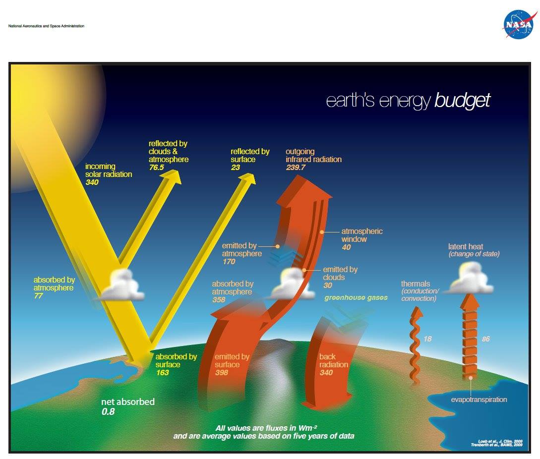
The surface energy budget then has the following form (image taken from the NASA Langley Research Center's website, Earth's Radiation Budget lithograph, 2016):


E(SFC) = SW↓ absorbed + LW↓ absorbed = LW↑ emitted + Turbulent↑
Energy (surface) = Solar Absorbed Surface + Downward Longwave Radiation = Upward LongWave + Sensible Heat +Latent Heat
For clear-sky:
E(SFC, clear) = SAS(clear) + DLR(clear) = ULW + (SH + LH)(clear)
and the same for all-sky.
The most important result we are going to present is the existence of certain relationships that connect the surface energy budgets to the TOA fluxes. This is not necessarily so: in general it is thought that the surface energy budget is a “free variable” of atmospheric downward emission (DLR) that in turn is depending on the atmospheric greenhouse gas amount. We show that, according to the data, there are specific constraints that determine the surface fluxes as variables of the TOA energy flows only.
Another fundamental flux element appears here: the difference of clear-sky and all-sky outgoing longwave radiations, which is the reduction of thermal emission of the Earth-system to space in the presence of clouds; it is called longwave cloud radiative effect (LW CRE); termed also the greenhouse effect of clouds. Some studies differentiate its TOA and SFC values (depending on the average cloud thickness); some regard them essentially the same (at least, within the error of observations).
Clouds are typically thick objects that block the way of infrared radiation therefore the most part of the cloud cover is thought to be effectively IR-opaque (except very thin clouds). The atmosphere itself is only partially opaque in the infrared: there is a so-called ‘atmospheric window’, where some part of the surface emission can pass directly to space (hence its name: Surface Transmitted Irradiance, STI).
So the clear-sky outgoing longwave radiation comes from two sources: upward emission from the atmosphere, and window radiation from the surface. In the all-sky mean: window radiation between the clouds, plus upward emission from the cloudy atmosphere. Note that window radiation and atmospheric emission cannot be observed: they can only be computed by radiative transfer codes. All the other quantities mentioned are observables: we use them from the said CERES data sources.
*
To our greatest surprise, there is a unique and unequivocal connection between the surface energy budget and the TOA fluxes, which for clear-skies looks like this:
By definition, OLR(clear) = OLR(all) + LWCRE, hence the equation can be written as:

According to the data, for the all-sky surface energy budget it is true that:

that is, E(SFC, clear) = E(SFC, all) + LWCRE.
We will show that, as a result, the internal fluxes in the all-sky global energy budget can be expressed as integer multiples of LWCRE, with a small difference which is less than one standard deviation for each fluxes:

The basic all-sky fluxes are:
Therefore, E(SFC, all) = 19 units and E(SFC, clear) = 20 units.
There is also a clear-sky structure, with specific relationship to the all-sly values:
![]()
Presenting detailed data and a possible theoretical framework is the main task of this webpage. We collected our results in a new global energy budget diagram and poster.
*
*
*
*
CONTENT
1. DATA
1.1 Clear-sky
Thermal Outgoing Radiation at top-of-atmosphere (TOA):
(all data in watts per square meter, W/m2, with about +/- 3 W/m2 uncertainty)
OLR(clear) = 265
Surface energy budget:
solar radiation absorbed plus downward atmospheric longwave radiation absorbed =
longwave emitted by the surface plus latent and sensible (turbulent) heat flux.
E(SFC) = SW↓ absorbed + LW↓ absorbed = LW↑ emitted + Turbulent↑
DATA FROM CERES Surface DQS:
SW down = 243.9
SW up = 29.7
SW absorbed = 214.2
LW absorbed = 316.0
LW emitted = 398.0
Turbulent = 132.2
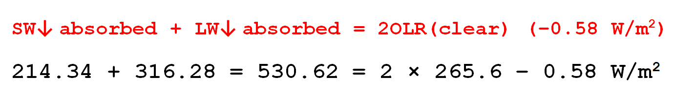
E(SFC) = 214 + 316 = 398 + 132 = 530.
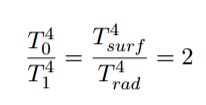
Let us realize: E(SFC, clear) = 2OLR(clear).
*
1.2 All-sky:
• Thermal Outgoing Radiation, all-sky, OLR(all) = 239.5
• SW absorbed + LW absorbed = LW emitted + turbulent
• 162 + 345 = 399 + 108 = 507
• Surface longwave cloud radiative effect, SFC LWCRE = 28
• 2OLR(all) + LWCRE = 507.
• E(SFC, all) = 2OLR(all) + LWCRE.
*
2. CONCEPTUAL FRAMEWORK:
2.1 Simplest greenhouse model: E(SFC) = 2OLR
2.2 Leaky greenhouse model: E(SFC) = 2OLR - LWCRE
2.3 Leaky greenhouse model with partial cloud cover: E(SFC) = 2OLR + LWCRE.
*
3. CONSEQUENCES
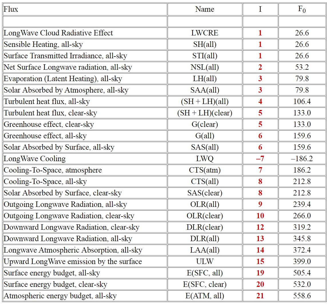
3.1 Quantized (integer) flux structure: F = F0 + ΔF, where F0 = N x UNIT, N is an integer, ΔF is a small difference
3.2 Planetary emissivity is constrained at f(all) = OLR(all)/ULW = 3/5
3.3 Greenhouse factors are predetermined at g(clear) = 1/3 and g(all) = 2/5
3.4 Planetary albedo has a steady state at α = 1 - sin 45° = 1 - √2/2 = 0.29289.
*
4. COMPLETE SOLUTION (OUR DIAGRAM AND POSTER)
*
5. DISCUSSION, FURTHER DIAGRAMS
*
6. CONCLUSIONS
*
SUMMARY
*
*
Surface energy budget of the Earth
1. DATA
*
E(SFC) = SW↓ absorbed + LW↓ absorbed = LW↑ emitted + Turbulent↑
*
E(SFC) = (SW down - SW up) + LW down
E
• CERES EBAF DATA
CLIMATE YEAR
![]()
![]()
![]()
CERES EBAF Ed2.8 Data Quality Summary (DQS) says:
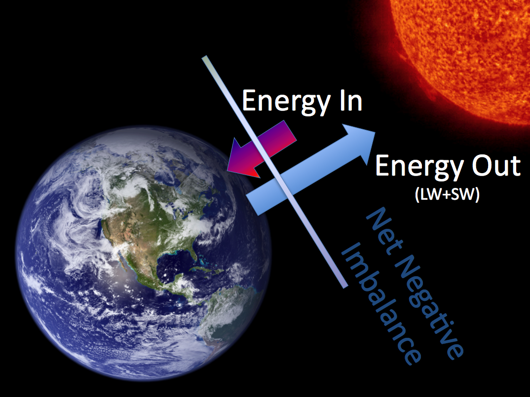
"Despite recent improvements in satellite instrument calibration and the algorithms used to determine SW and LW outgoing top-of-atmosphere (TOA) radiative fluxes, a sizeable imbalance persists in the average global net radiation at the TOA from CERES satellite observations. With the most recent CERES Edition3 Instrument calibration improvements, the SYN1deg_Edition3 net imbalance is ~3.4 W m-2, much larger than the expected observed ocean heating rate ~0.58 W m-2 (Loeb et al. 2012a).
"The CERES Energy Balanced and Filled (EBAF) dataset uses an objective constrainment algorithm to adjust SW and LW TOA fluxes within their ranges of uncertainty to remove the inconsistency between average global net TOA flux and heat storage in the Earth-atmosphere system."
"In the current version, the global annual mean values are adjusted such that the July 2005–June 2010 mean net TOA flux is 0.58 ± 0.38 W/m2."
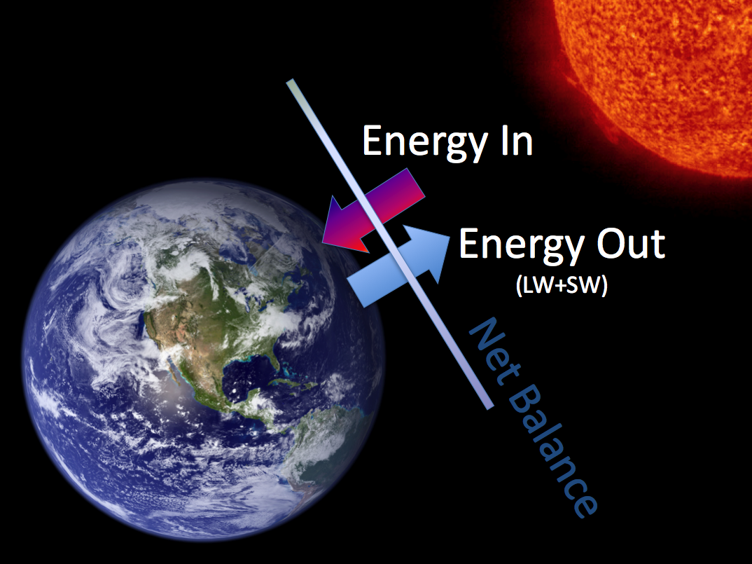
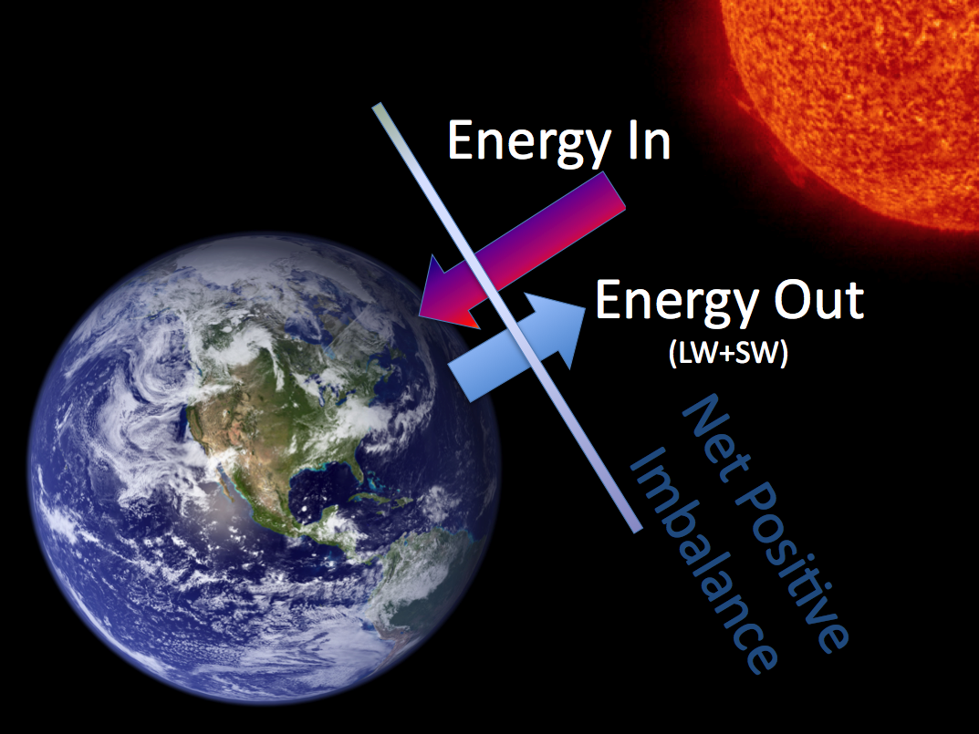
CERES EBAF Net Balancing web page says:
- "For the Earth to remain in balance the energy coming into and leaving the Earth must equal.
- The
CERES absolute instrument calibration currently does not have zero net
balance and must be adjusted to balance the Earth's energy
budget". The concept is illustrated by the following pictures (credit NASA LaRC):
It is evident that 'data' here does not mean raw data, but data products, adjusted, optimized and second-optimized to satisfy several constraints: precipitation, water cycle, energy cycle, ocean heat content, net TOA and surface energy budgets.
These adjustments are generally well-documented. But we were not able to find any documentation about adjustments to the E(SFC, clear) = 2OLR(clear) equality.
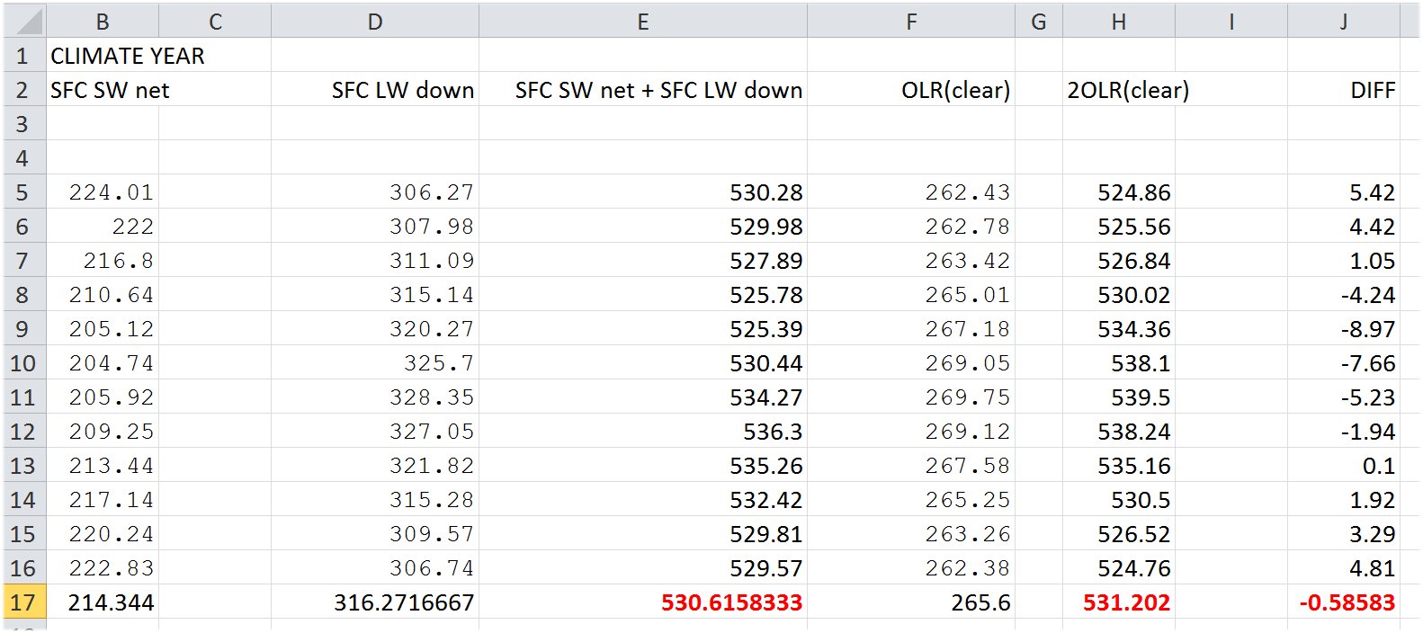
DIFF = -0.58 W/m2 results from adjustment to
ASR = OLR + 0.58 W/m2.
Taking this value into account,
the following equality becomes exactly true:
E(SFC, clear) = SW absorbed + LW absorbed = 2OLR(clear).
*
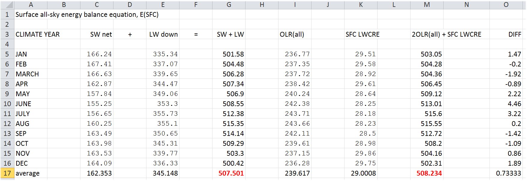
Detailed data for time period 2001 - 2015
*
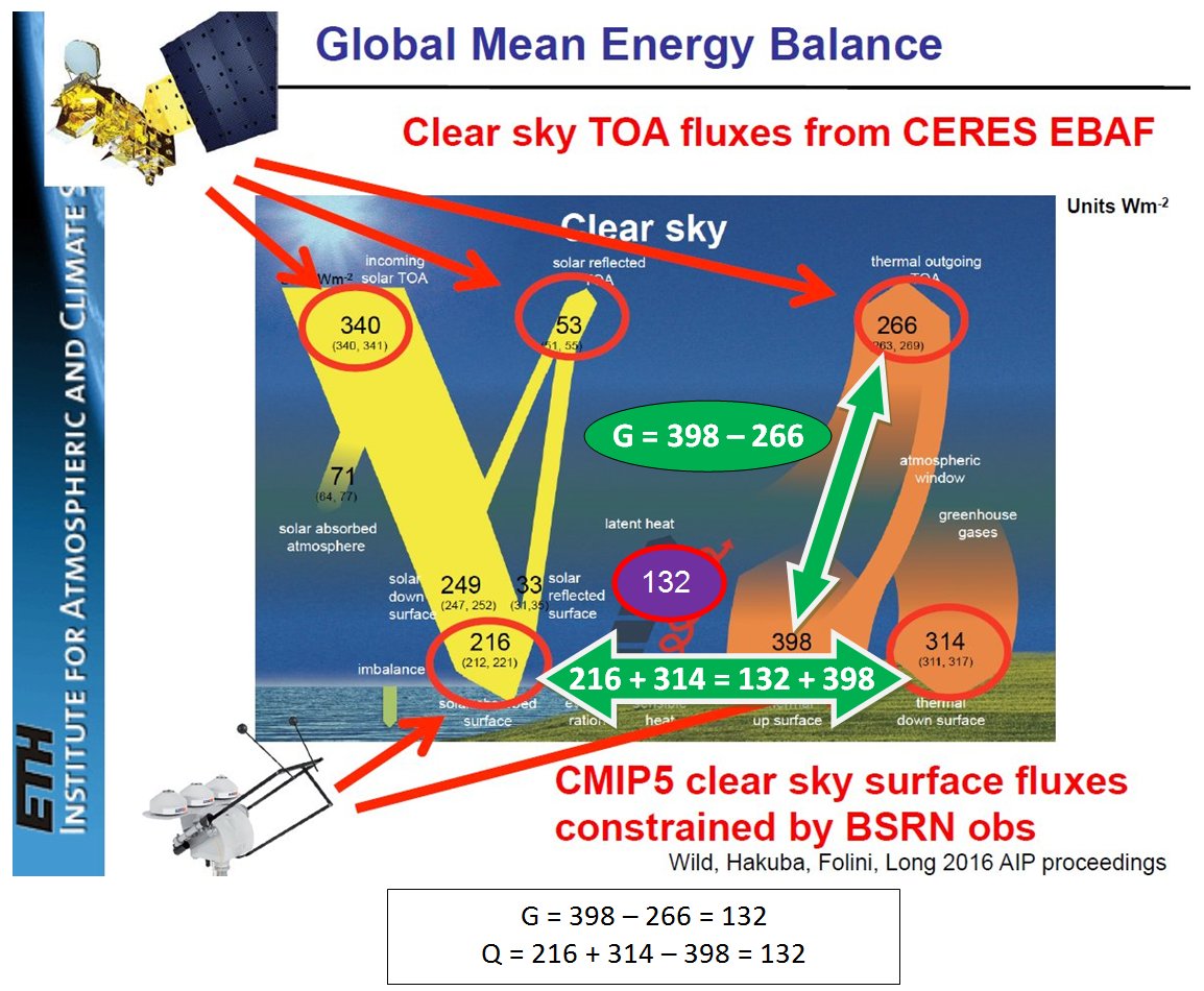
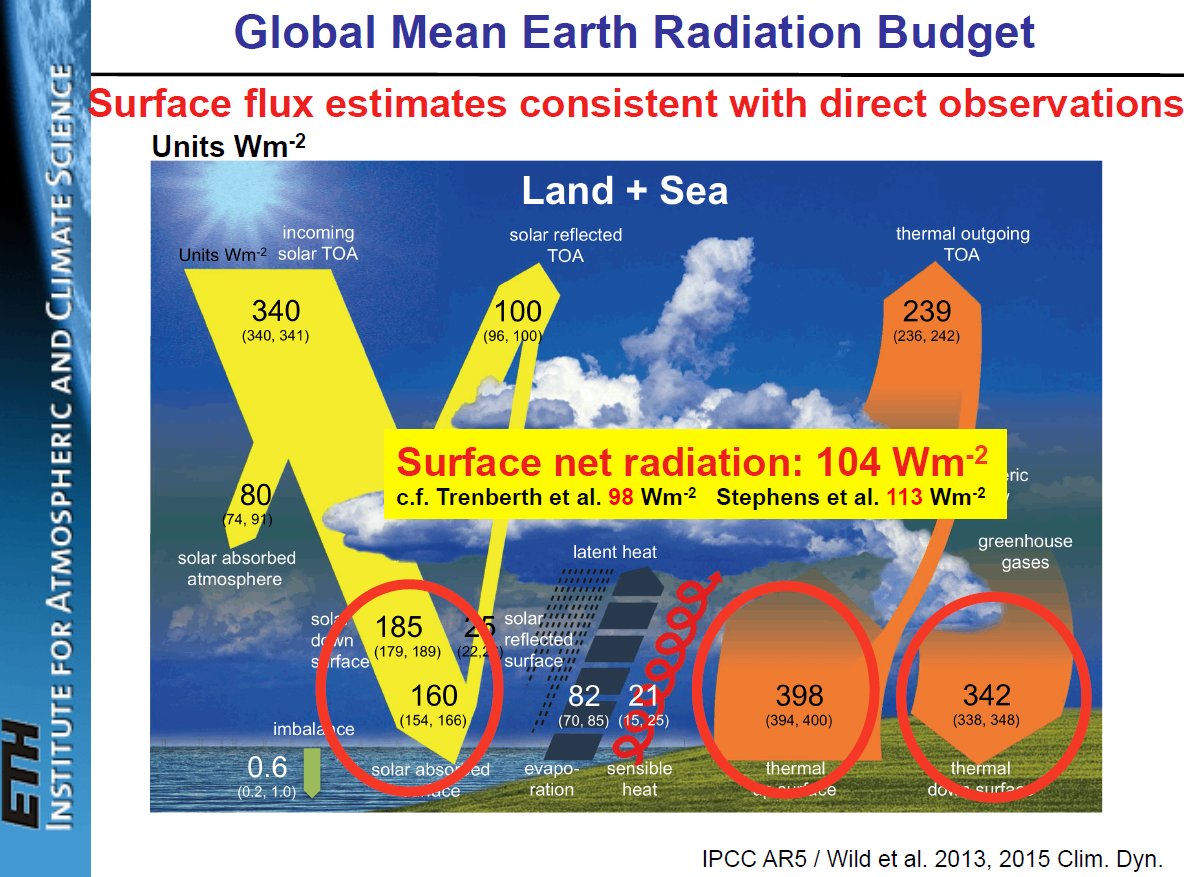
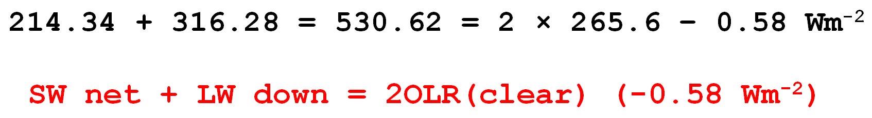
The slide below is from a CERES Science Team Meating presentation (Martin Wild, Oct 2016).
Our addition in green, below the frame.
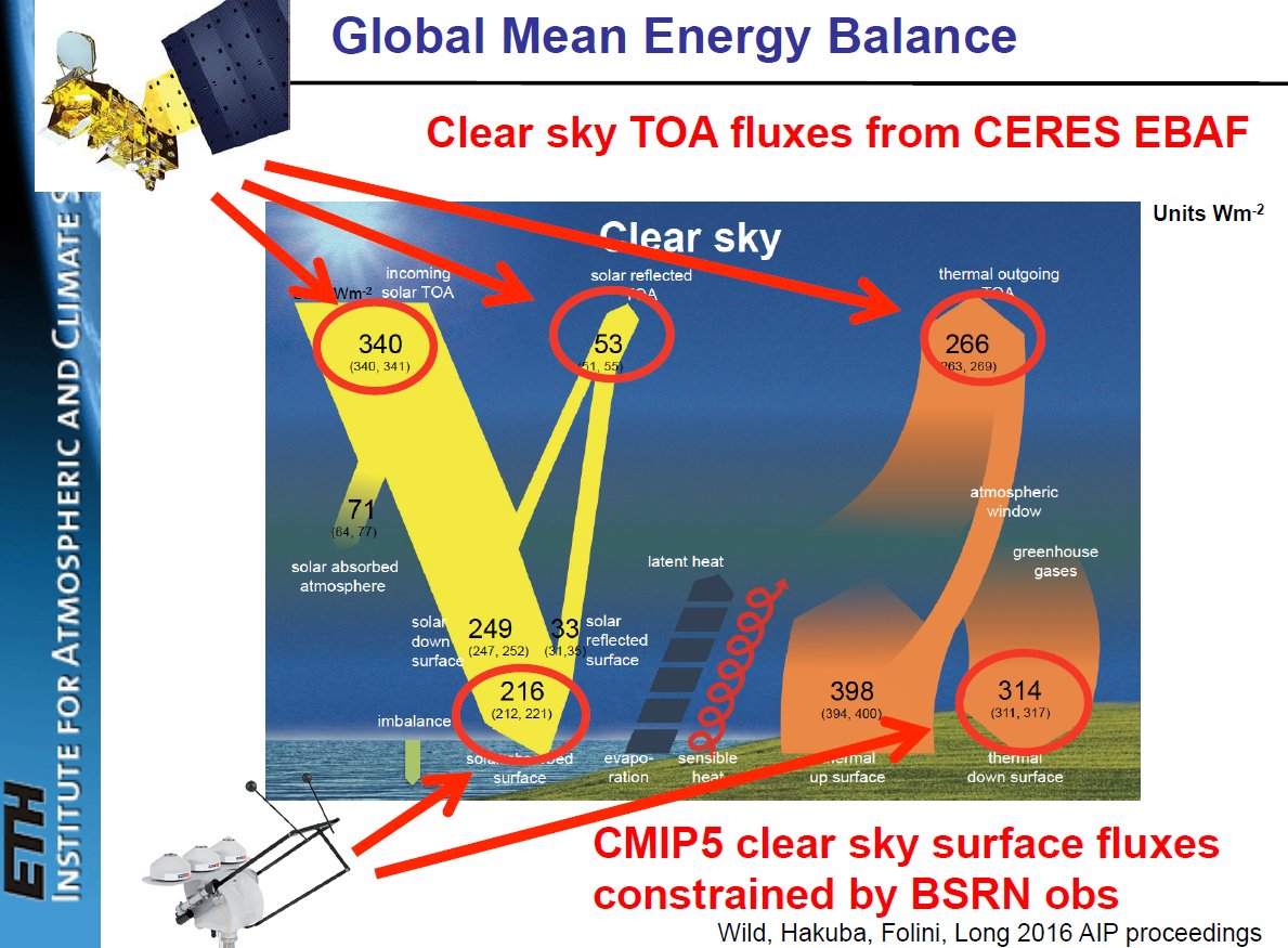
As the diagram says,
the two sides of the equality come from different observational sources.
Data on the left-hand side (surface) come from CMIP5 fluxes constrained by BSRN observations;
data on the right hand side (TOA) come from CERES.
And still, as it can be seen, they are rigorously interconnected:
216 + 314 = 530 ( + imb) = 2 × 266 ( -1)
*
![]()
E(SFC, clear) = SW absorbed + LW absorbed = 2OLR(clear)
far within the observation error (+/- 5 Wm-2).
***
Is this a general planetary rule?
Not at all.
In the thin, full-CO2 Martian atmosphere
the energy absorbed by the surface is much less than twice the OLR:
![]()
Original: Read et al. (2015), our additions in boxes
E(SFC, Mars, clear) = SW abs + LW abs = 96 + 27 = 123 W/m2.
2OLR(clear, Mars) = 220 W/m2
E(SFC, Mars, clear) << 2OLR(clear).
*
The simplest greenhouse model
This relationship:
E(SFC) = 2OLR
is the trivial solution of radiative transfer for the simplest greenhouse model,
comprising a planetary surface surrounded by a thin SW-transparent, LW-opaque "closed glass shell".
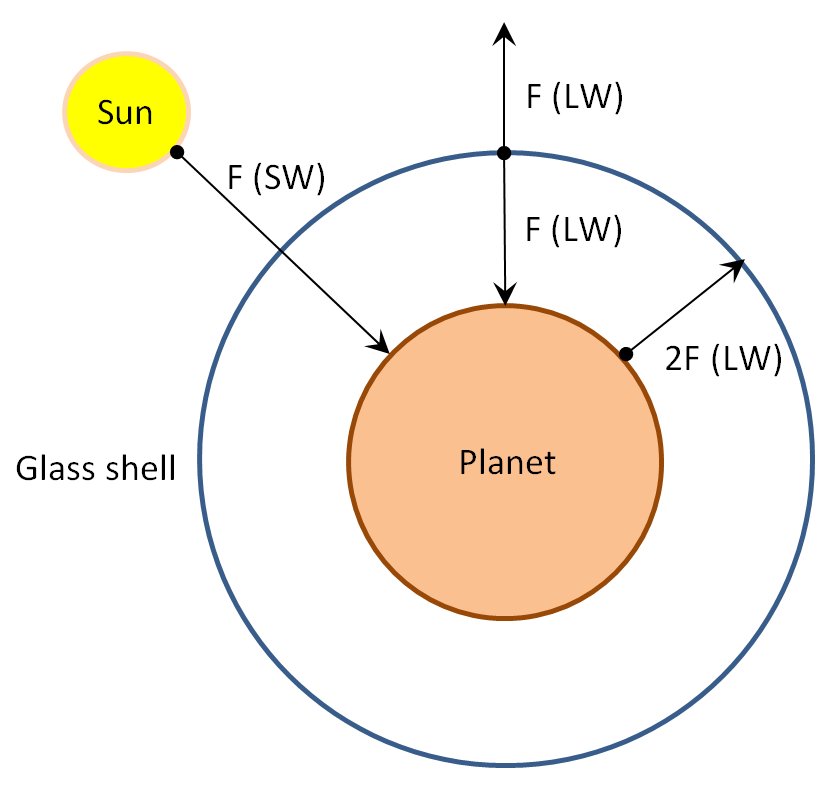
The shell radiates in all directions equally so that half goes up, F(LW) = OLR, and half goes down, F(LW) = DLR: OLR = DLR. Because the half that goes up must be equal to the incoming solar flux, F(SW), the total flux from the surface is equal to twice the outgoing radiation flux.

An easy-to-follow description of this model is given for example in the textbook of Marshall and Plumb (2008), Chapter 2: The global energy balance, Section 2.3. The greenhouse effect, Figure 2.7. and equation 2-8 below:
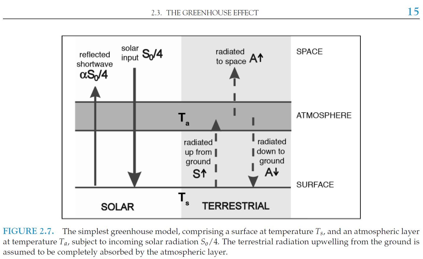
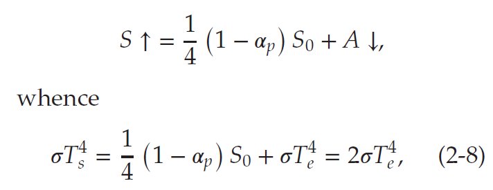
as shown here:
The terrestrial radiation upwelling from the ground is assumed to be completely absorbed by the glass shell.
Highest absorption model:
E(SFC) = 2OLR
Another textbook representation (D. Dommenget, Oct 2016):
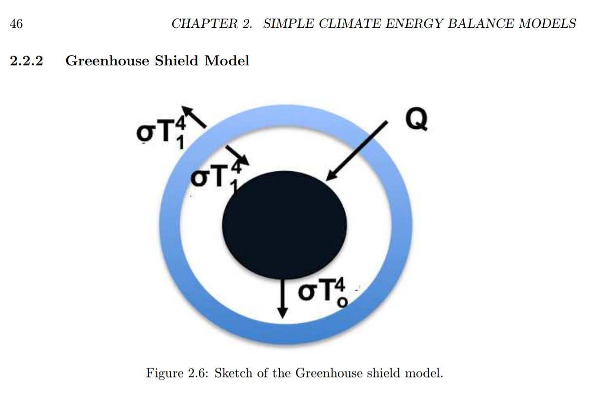
 =>
=> 
Wikipedia: 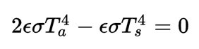 Factor 2 is resulting from the geometry.
***
Or another
(Elementary Climate Physics, F. W. Taylor):
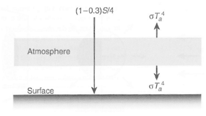
Fig. 7.4. A 'single-slab model' of the greenhouse effect.
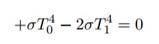
TOA:
(1–0.3)S/4 =σTa4
Surface:
(1–0.3)S/4 + σTa4 = σTs4
so
2σTa4 = σTs4 .
(Spherical area difference: 0.9 W/m2)
***
Leaky greenhouse, clear sky
Observed data:
E(SFC, clear) = LW up + Surface net = 398.0 + 132.2 W/m2
Outgoing LW TOA: Opaque part + Leaky part
OLR(clear) = ATM(clear) + WIN(clear) = 265.7 W/m2
WIN(clear) is 'Atmospheric Window' = 66 W/m2
(Costa and Shine 2012), hence
ATM(clear) is 'Emitted by Atmosphere' = 199.7 W/m2
*
Surface LW up = 2 ATM(clear),
Surface net (G) = 2 WIN(clear)
***
![]()
***
Leaky, turbulent clear-sky
The 2Ta4 = Ts4 relationship above assumes (requires) that the
planetary surface and the shell are isolated, that is, NO
any other energy transfer (physical contact) exists between the two than radiation.
In reality, the atmosphere is in contact with the planet,
and there are convective / conductive energy flows:
sensitive and latent (turbulent) heat fluxes
between the Earth's surface and the emitting atmospheric layer.
If WIN is lost at TOA, then 2 WIN is missing from the surface: *
ULW = E(SFC) – 2 WIN,
hence
Surface net (turbulent flux) = 2 WIN.
As a result,
E(SFC, clear) = 532 W/m2, ULW = 399 W/m2, OLR(clear) = 266 W/m2,
ATM(clear) = 199.5 W/m2, Turb = 133 W/m2 and WIN(clear) = 66.5 W/m2.
Ratios:
8 / 6 / 4 / 3 / 2 / 1.
The clear-sky greenhouse effect is
G = ULW – OLR = Turb (= Net SFC = SH + LH = Q) = 2 UNITS = 133 W/m2
E(SFC, clear) = ULW + G(clear) = 2OLR(clear)
DATA:
![]()
![]()
We are not aware of any expert description of the clear-sky greenhouse effect as the sum of the sensible and latent fluxes.
ULW + G = 2OLR (- 0.01 W/m2).
If ULW + G is constrained to 2OLR,
ULW + G can be increased only if OLR increases.
***
*
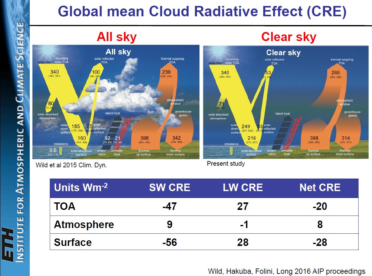
All-sky
Data from CERES DQS
Surface
SW down = 186.4 (+/-5) W/m2
SW up = 24.1 (+/-3) W/m2
LW down = 345.1 (+/-7) W/m2
Surface energy absorbed = SW down - SW up + LW down
= SW abs + LW down =
186.4 - 24.1 + 345.1 = 507.4 W/m2.
TOA outgoing LW = 239.6 W/m2.
507.4 = 2 x 239.6 + 28.2.
Long Wave Cloud Radiative Effect at the surface, SFC LWCRE
(known also as The greenhouse effect of clouds):
SFC LWCRE = 345 - 316 = 29 (W/m2)
E (SFC, all) = 2OLR(clear) - LWCRE = 2OLR(all) + LWCRE
(-0.73 W/m2)
(Spherical area difference: ~0.9 W/m2.)
*
*
LWCRE, Longwave cloud radiative effect: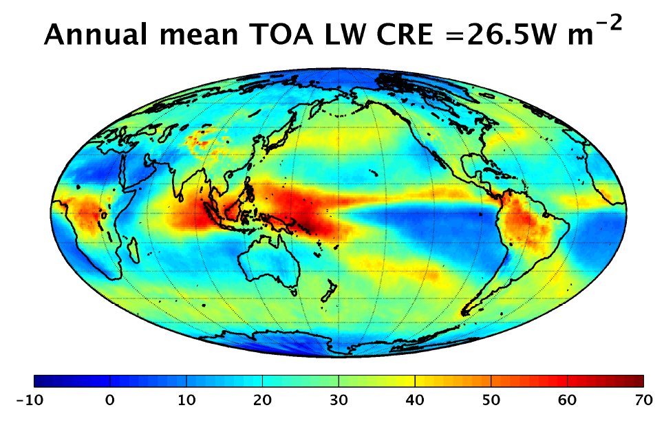 | 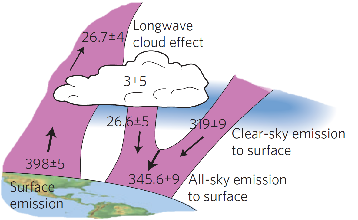 |
***
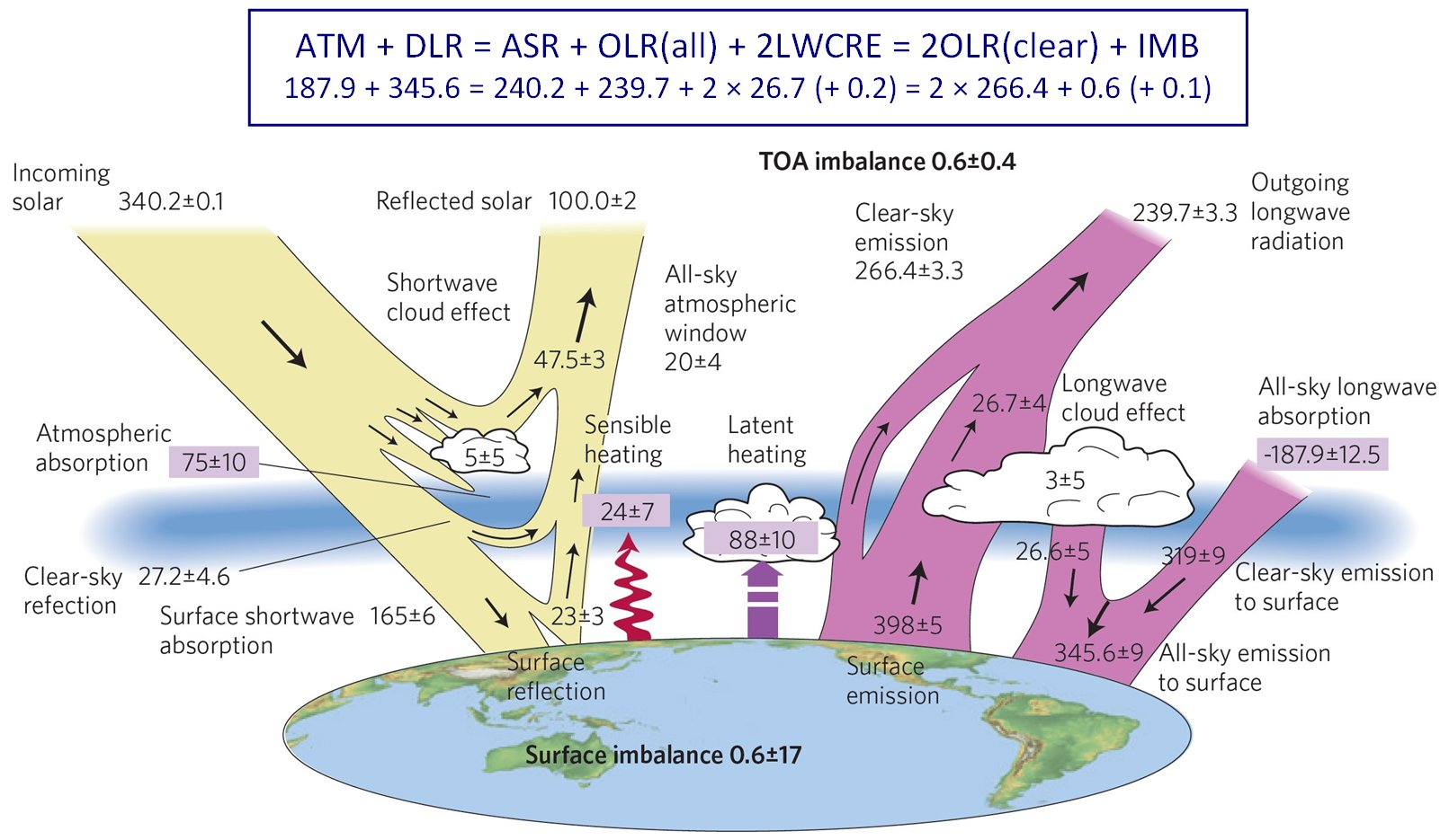
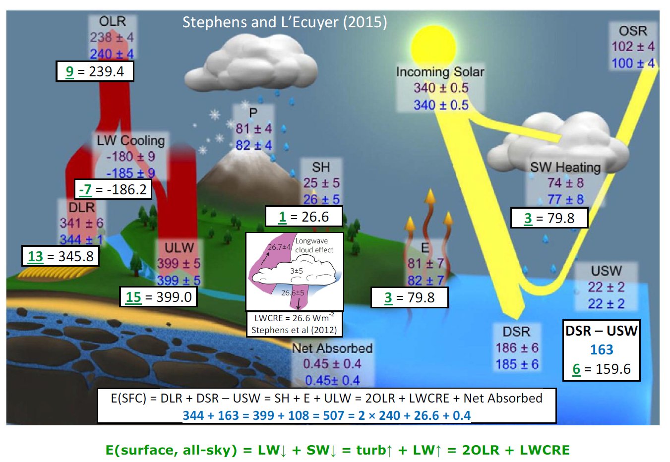
The all-sky relationship for Earth can be seen also in the latest published energy budget study of
Stephens and L'Ecuyer 2015:
Surface:
SW absorbed = 185 - 22 = 163 W/m2
LW absorbed = 344 W/m2
OLR = 240 W/m2
LWCRE = 26.6 W/m2
163 + 344 = 507 = 2 x 240 + 26.6 + 0.4
E(SFC,
all) = 2OLR(clear) - LWCRE = 2OLR(all) + LWCRE +IMB
The difference is 0.05 W/m2.
The fit seems to be resulting from adjustment.
*
Contrary to all differences, the semi-transparent, turbulent atmosphere of the Earth still follows the simplest greenhouse model.
Every element work in the direction to mimic the glass shell geometry; with the greenhouse effect
of a partial cloud cover
(LWCRE), the result is the same:
Clear-sky: Energy (SFC, clear) = 2OLR(clear) = 2OLR(all) + 2LWCRE All-sky: Energy (SFC, all) = OLR(clear) + OLR(all) = 2OLR(clear) - LWCRE = 2OLR(all) + LWCRE Cloudy-sky: Energy (SFC, cloudy) = OLR(clear) + OLR(cloudy).
|
***
ATMOSPHERIC VERSION
of these relationships can be recognized in the updated energy
balance diagram of
Stephens et al. 2012, Nat Geosci (our addition is in the textbox):
The difference is 0.1 W/m2.
The fit again seems to be resulting from adjustment.
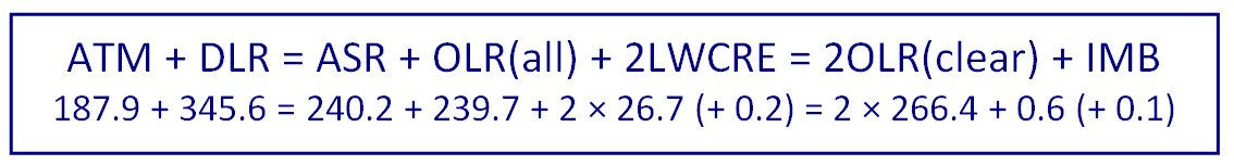
The atmospheric energy budget is unequivocally connected to the TOA fluxes.
We were not able to find any publicly available documentation for this equality.
***
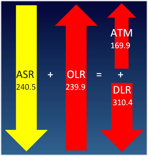
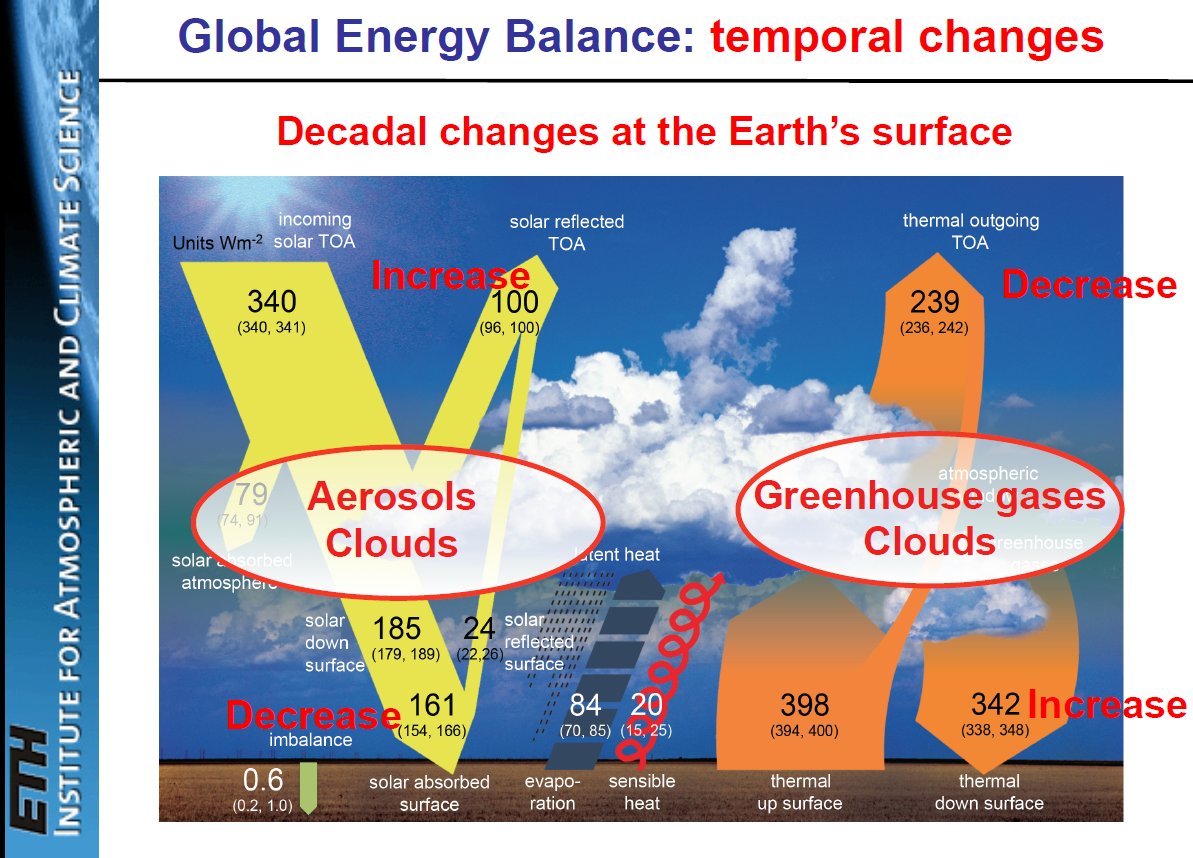
The same can be observed also in the NASA Langley Research Center's Global Energy Budget poster, 2014 June (our additions: yellow and red arrows and white text boxes):
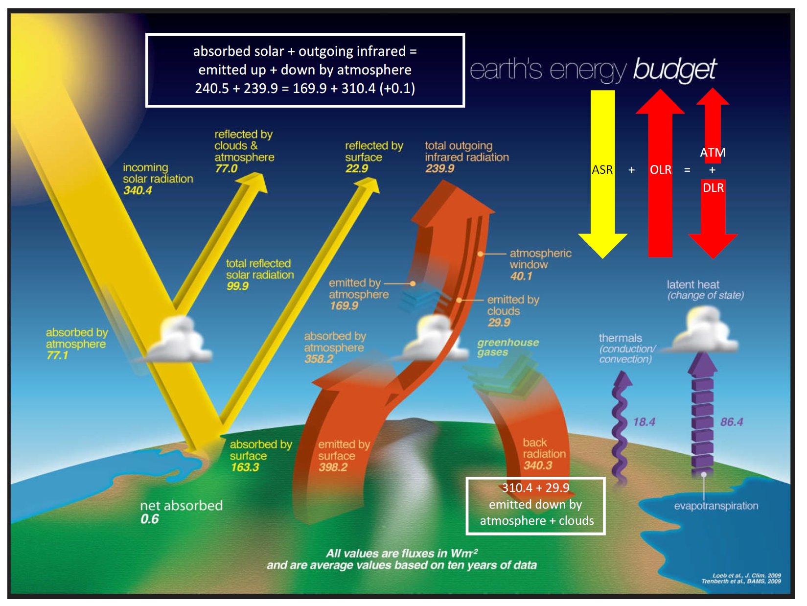
ASR:
Absorbed Solar Radiation; OLR: Outgoing Longwave Radiation; ATM: Atmospheric upward emission;
Back radiation: emitted down by atmosphere and clouds.
DLR: Downward Longwave Radiation by atmosphere only.
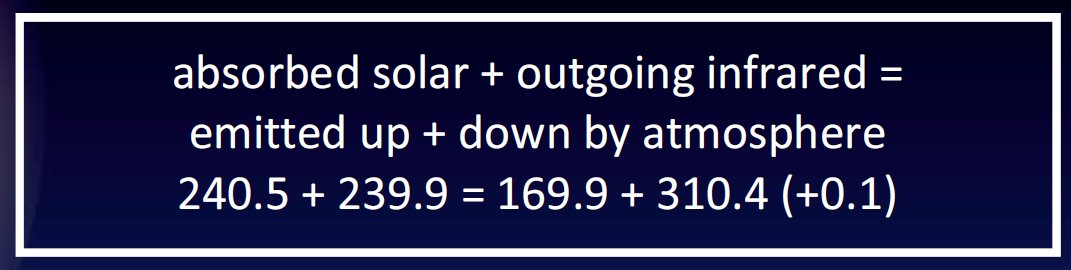
According to the data of this poster, it is valid within 0.1 W/m2:
Emitted by atmosphere (up) + back radiation = ASR + OLR + emitted by clouds
(169.9 + 340.3 = 240.5 + 239.9 + 29.9)
The atmospheric energy budget is constrained to the energy flows at TOA:
It is evident that this is NOT the case in the Martian thin, full-CO2 atmosphere:
![]()
***
The surface and atmospheric energy budgets of Earth seem to be
not internally
determined by the atmospheric trace gas (greenhouse gas) composition;
they are entirely regulated by the geometry.
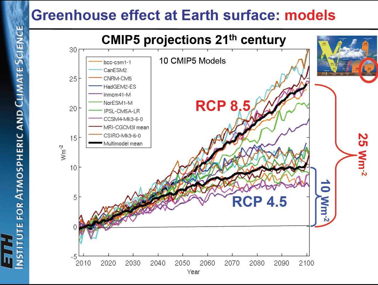
The equalities above sharply contradict Figure S2 of the Supplementary Information to the Stephens et al. (2012) paper:
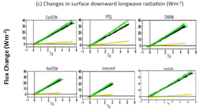
showing simulated increase of 30 W/m2 in DLR to the end of this century;
displayed also in this WMO presentation by one of the authors:
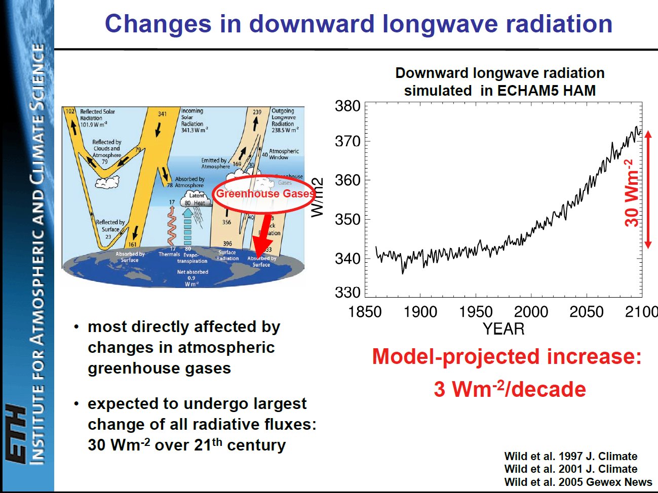
further, it contradicts the UN IPCC AR5 (2013) Chapter 8 opening statement:
"It is unequivocal that anthropogenic increases in the well-mixed
greenhouse gases (WMGHGs) have substantially enhanced
the greenhouse effect",
since the equations describe that the total (upward plus downward) atmospheric emission is constrained to the boundary conditions.
Therefore, the greenhouse effect can be enhanced only by
increasing absorbed solar radiation (ASR).
***
3. CONSEQUENCES
1.
QUANTIZED (INTEGER) flux structure
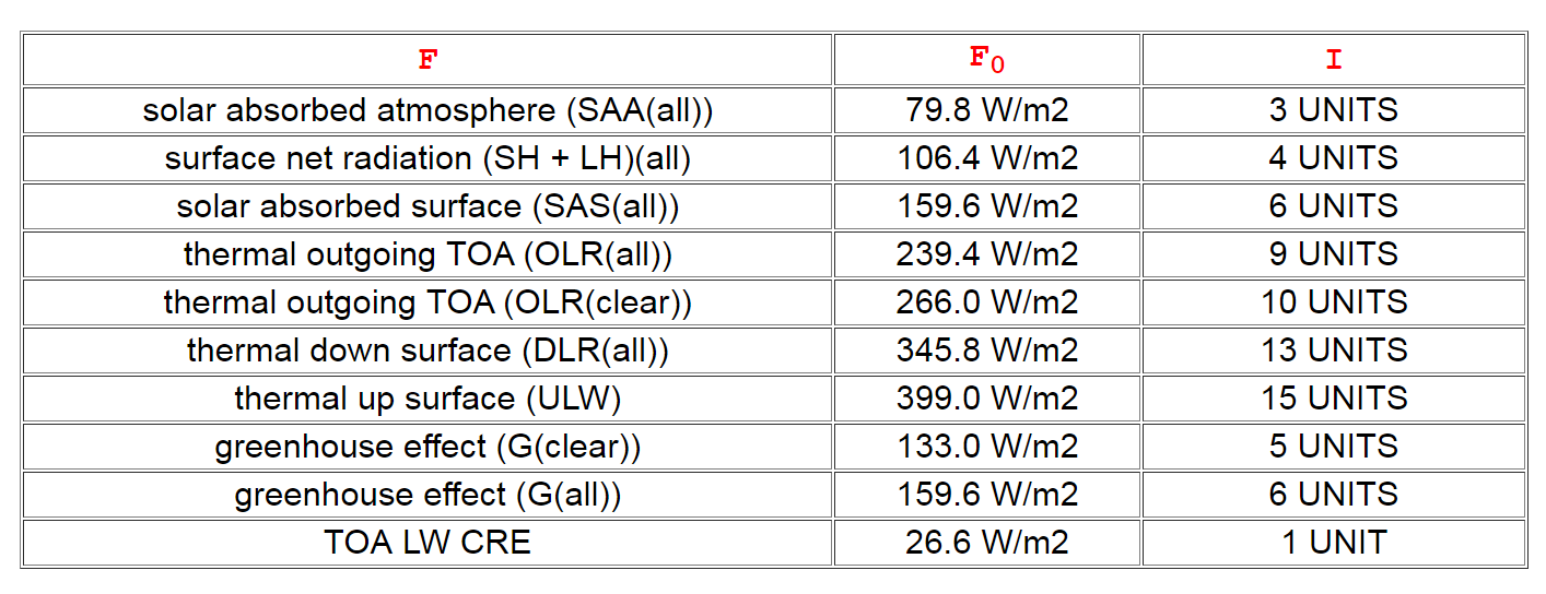
UNIT = ASR/9 (- 0.6 W/m2 imbalance)
*
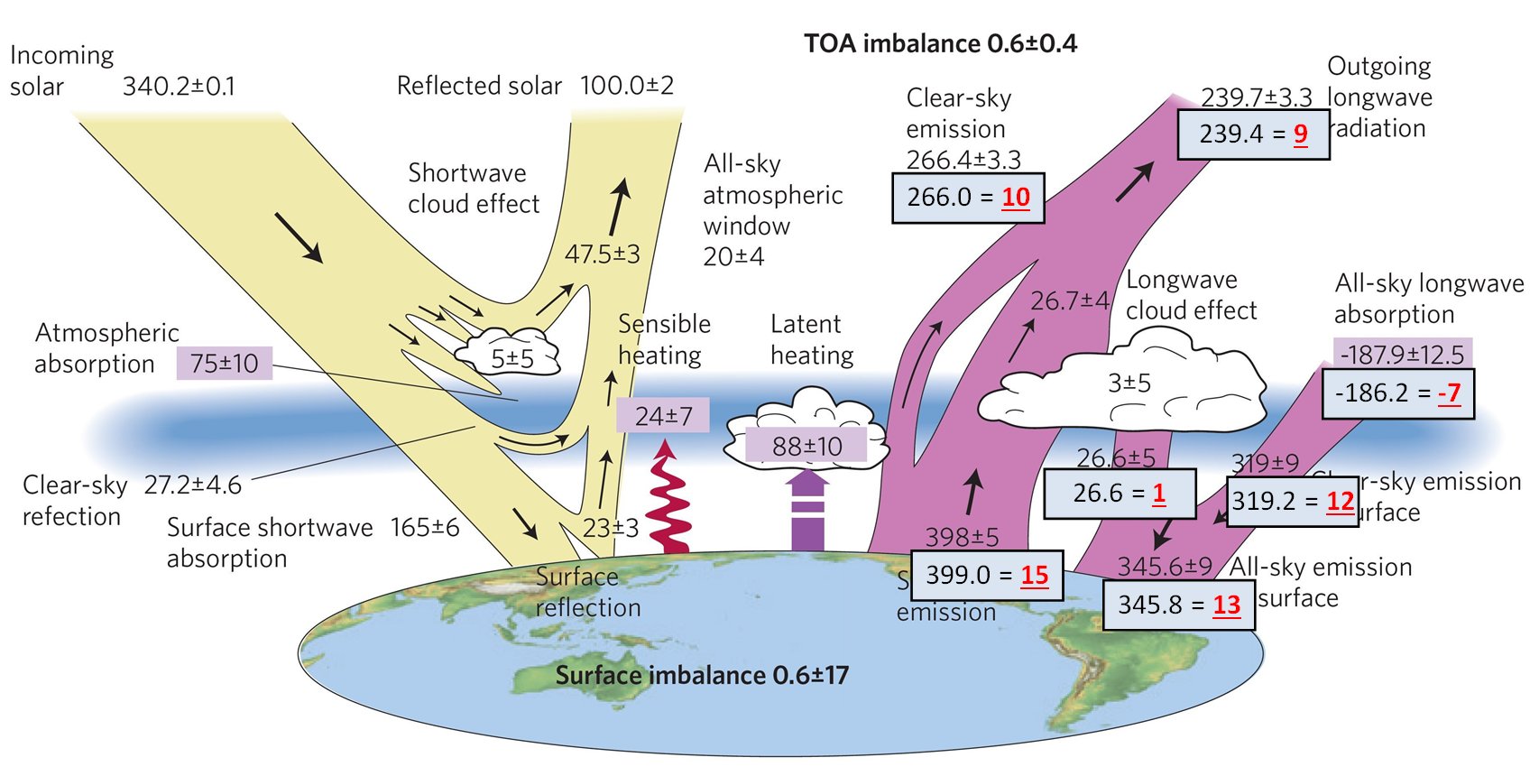
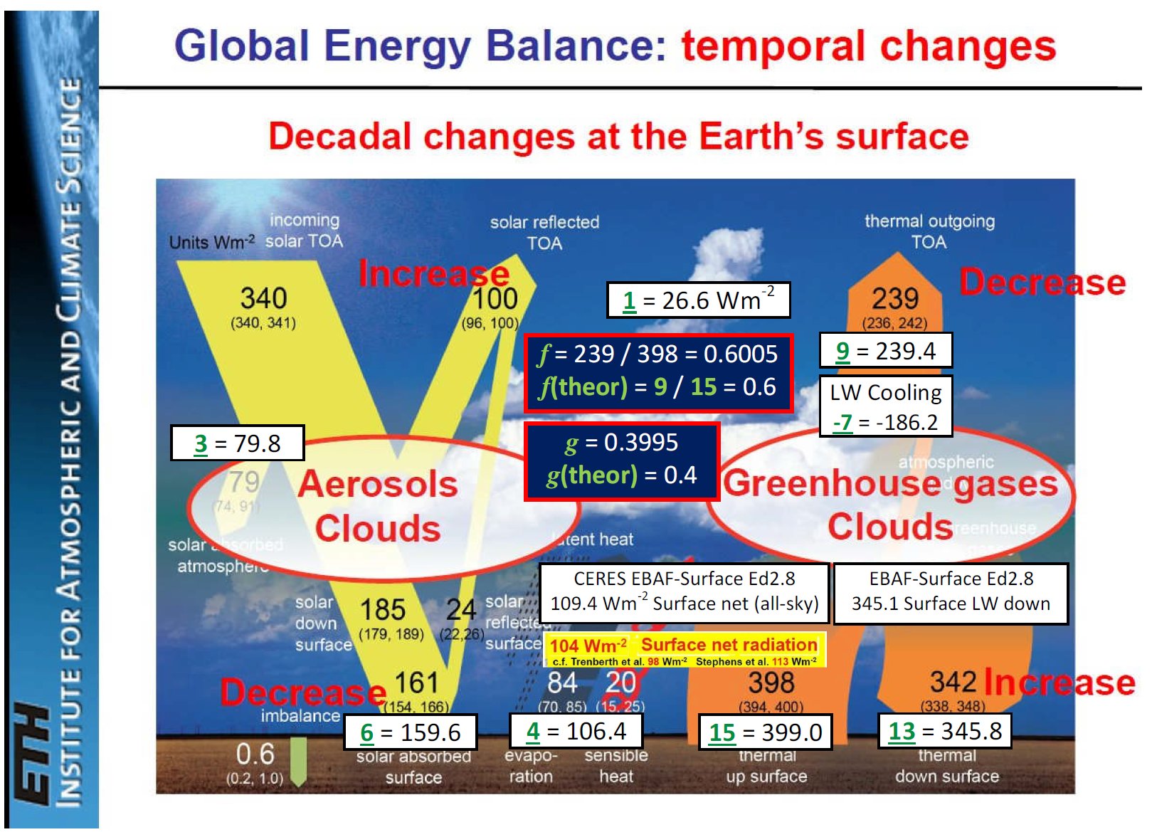
| LWCRE = | 1 × 26.6 = | 26.6 W m-2 = | 1 |
| SW Heating = | 3 × 26.6 = | 79.8 W m-2 = | 3 |
| SH + E = | 4 × 26.6 = | 106.4 W m-2 = | 4 |
| SW Absorbed = | 6 × 26.6 = | 159.6 W m-2 = | 6 |
| OLR = | 9 × 26.6 = | 239.4 W m-2 = | 9 |
| OLR(clear) = | 10 × 26.6 = | 266.0 W m-2 = | 10 |
| DLR = | 13 × 26.6 = | 345.8 W m-2 = | 13 |
| ULW = | 15 × 26.6 = | 399.0 W m-2 = | 15 |
| LW Cooling = | -7 × 26.6 = | -186.2 W m-2 = | -7 |
*
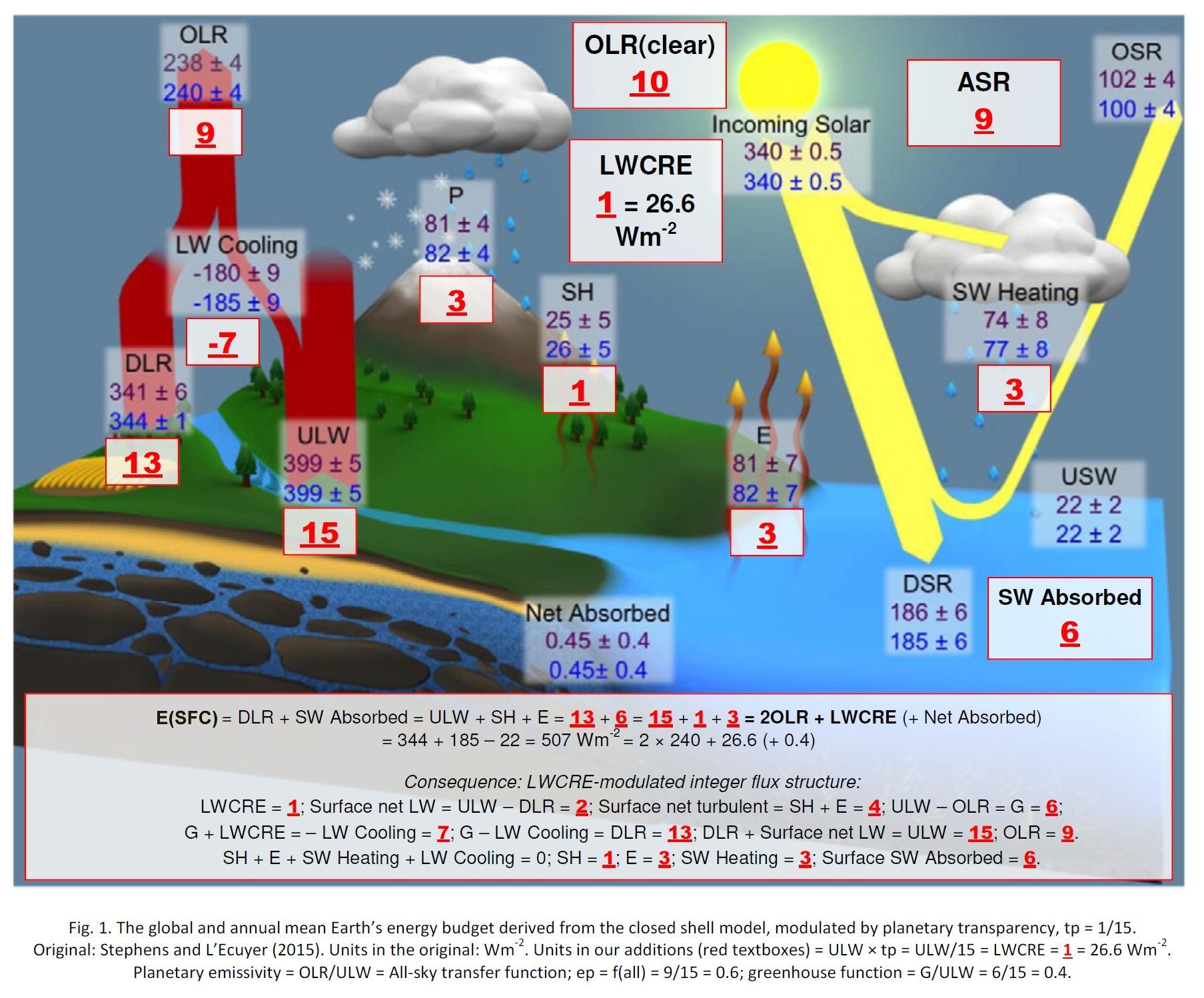
LW integer structure projected on Stephens et al. (2012)
(our additions in the textboxes):
Stephens and L'Ecuyer (2015), based on the assessment of L'Ecuyer et al. (2015),
applied relevant water cycle constraints (latent heat adjustment);
the result is an integer structure for all fluxes
(our additions: textboxes in the diagram, equations below, and figure legend):
*
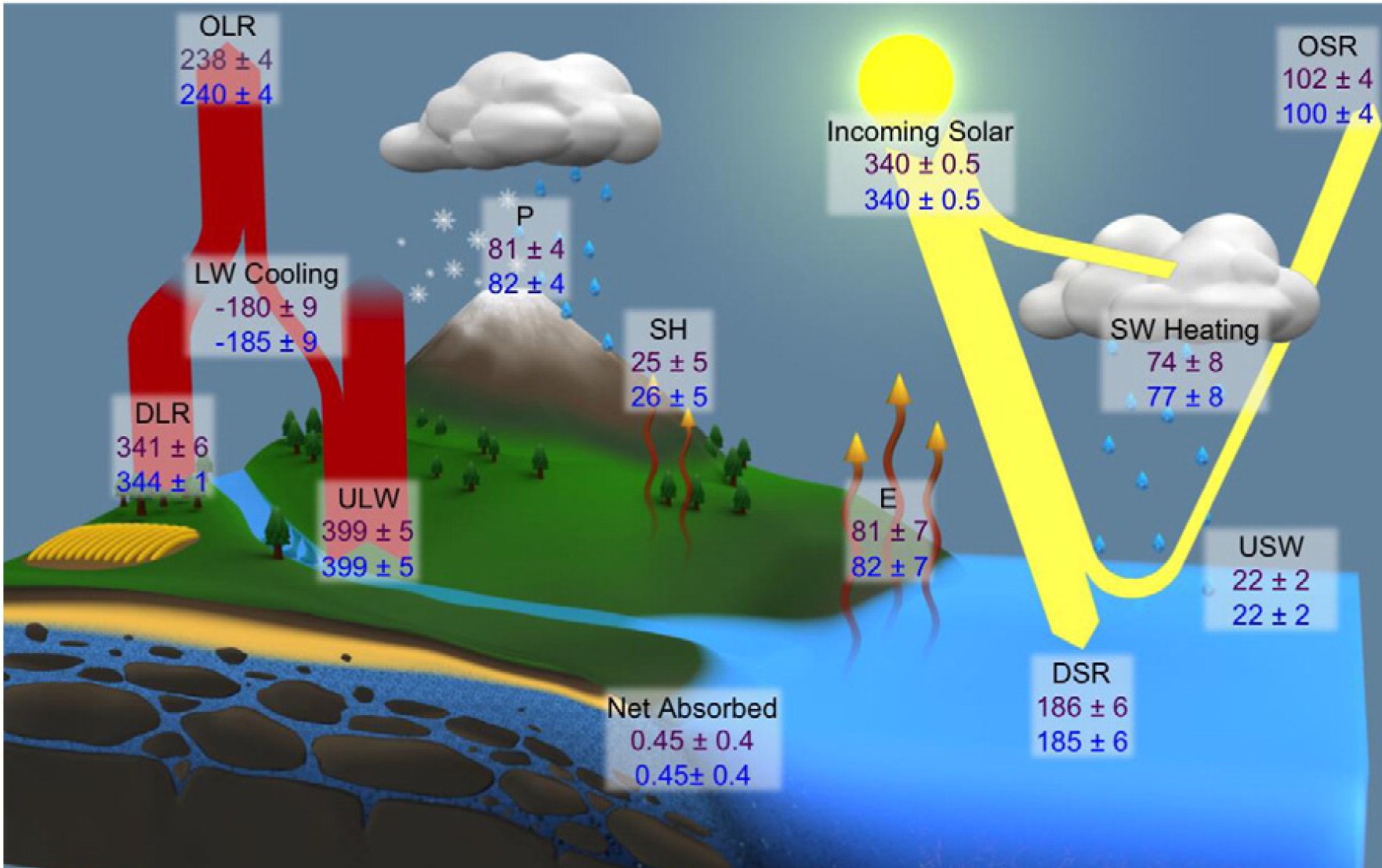
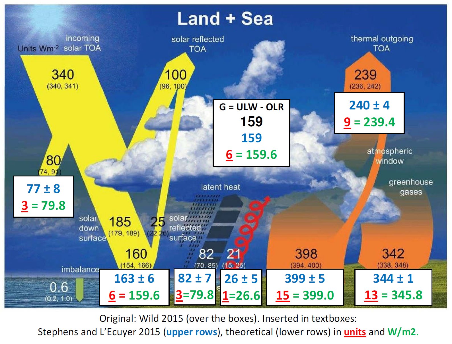
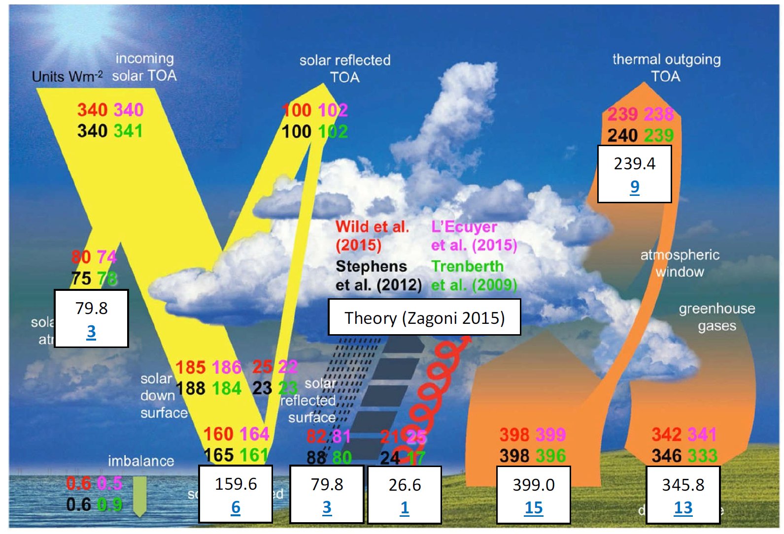
The integer structure projected on the Wild et al. (2015) diagram:
Wild et al. (2015)
Stephens and L'Ecuyer (2015) (in blue)
our model (units in red and W/m2 in green)
To
get a better understanding of the LWCRE-modulated integer flux structure, solve the
Climate Sudoku:

Hint: ASR = 9 = 240 W/m2 - IMB. Calculate the surface and atmospheric energy balance!
(LWCRE = 1 = 26.6 W/m2)
Surface: SW abs + LW abs = LW up + Turbulent
Atmosphere: SW abs + LW abs + Turbulent = LW emitted up + LW emitted down
*
Solution:
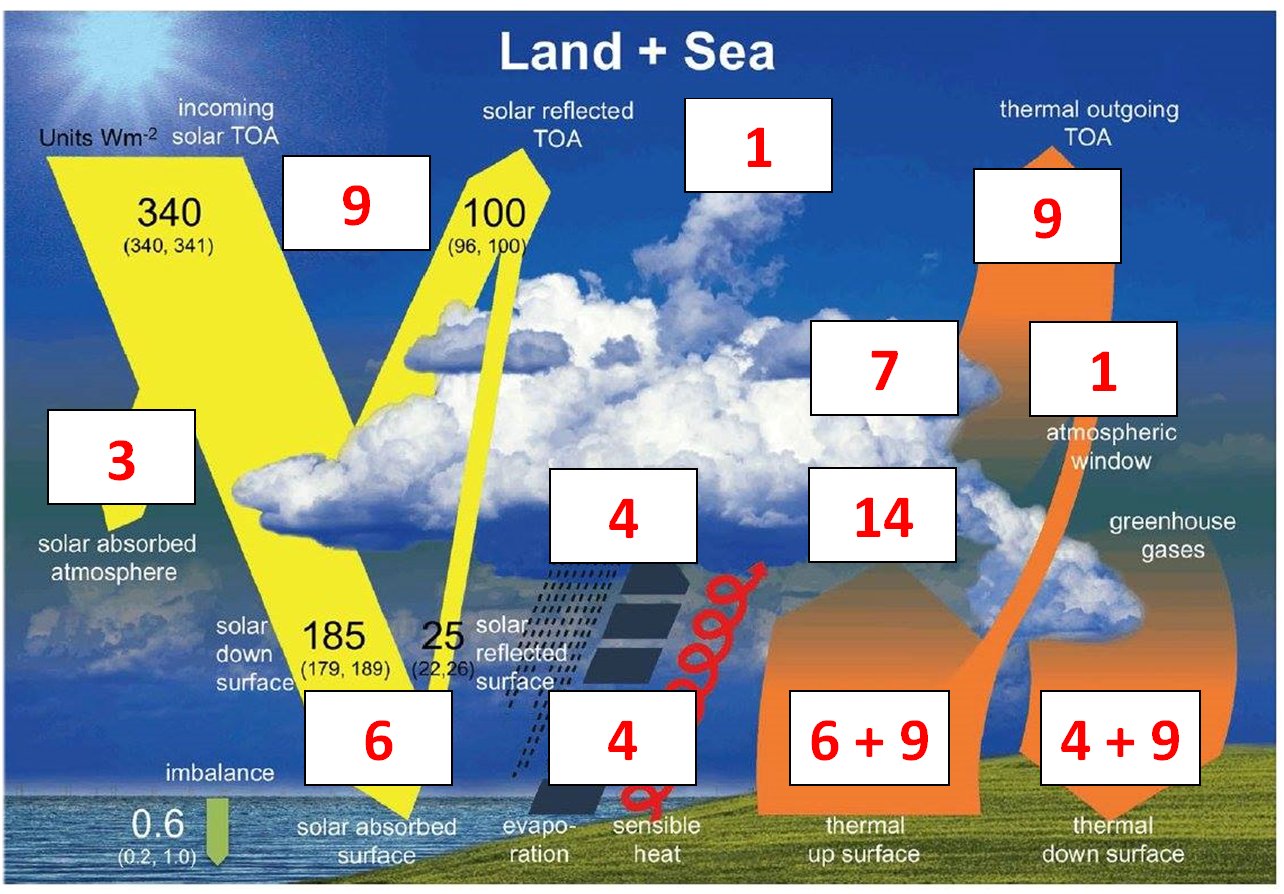
Source of the diagram: Wild et al. (2015) Clim Dyn
Source of the data: NASA CERES
Red: UNITS, Green: W/m2
***
2.
Planetary emissivity is constrained at ep = f(all) = 3/5
f(all) = OLR(all)/ULW
CERES DATA TIME PRIOD 2001 - 2015:
ULW:
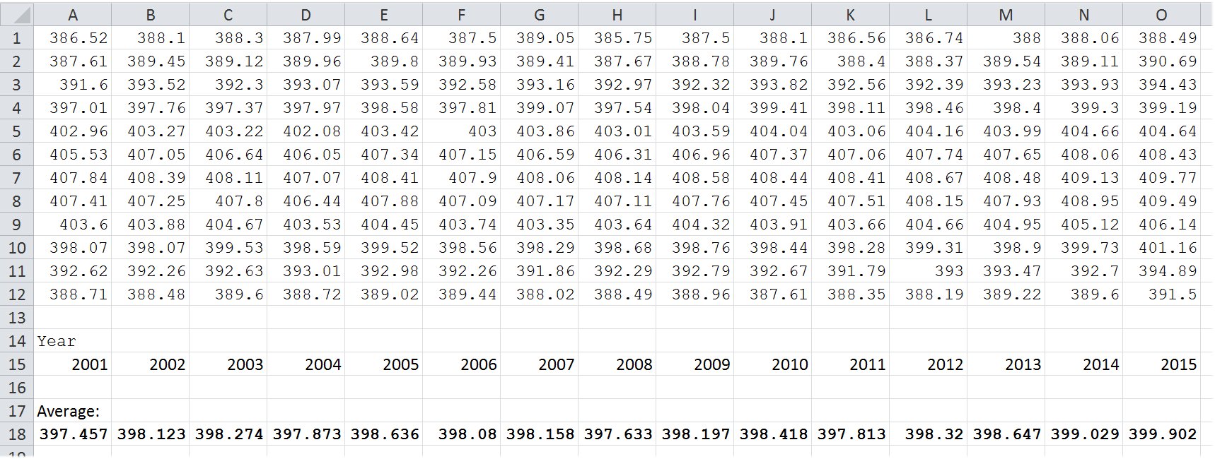
OLR(all) and f(all):
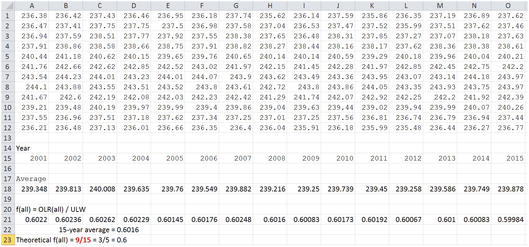
Average of 15 years :
ep(all) = f(all) = 0.6016
Theoretical: f(all) = 0.6
3.
The normalized all-sky greenhouse factor is stable at g(all) = 2/5,
the clear-sky greenhouse factor is stable at g(clear) = 1/3.
The greenhouse effect is defined as the difference of the two boundary LW radiations: G = surface upward longwave emission minus TOA outgoing LW radiation, G = ULW - OLR, and the normalized greenhouse factor is g(all) = G(all) / ULW. With OLR(all) = 239.4 W/m2 and ULW = 399 W/m2, we have g(all) = 2/5 = 0.4. This value is pre-determined by the pattern, and cannot change (except tiny fluctuations, 'vibrations' - with unknown size and time-scale). There is no enhanced (elevated, increased) greenhouse effect from change in the atmospheric trace-gas composition.
g(clear) = G(clear) / ULW = 1/3 is equivalent to:
Clear-sky planetary emissivity ep(clear) = clear-sky transfer function =
f(clear) = OLR(clear) / ULW = 2/3.
CERES DATA TIME PRIOD 2001 - 2015:
ULW:
OLR(clear) and f(clear):
![]()
Average of 15 years :
ep(clear) = f(clear) = 0.666761.
Theoretical: f(clear) = 0.666666.
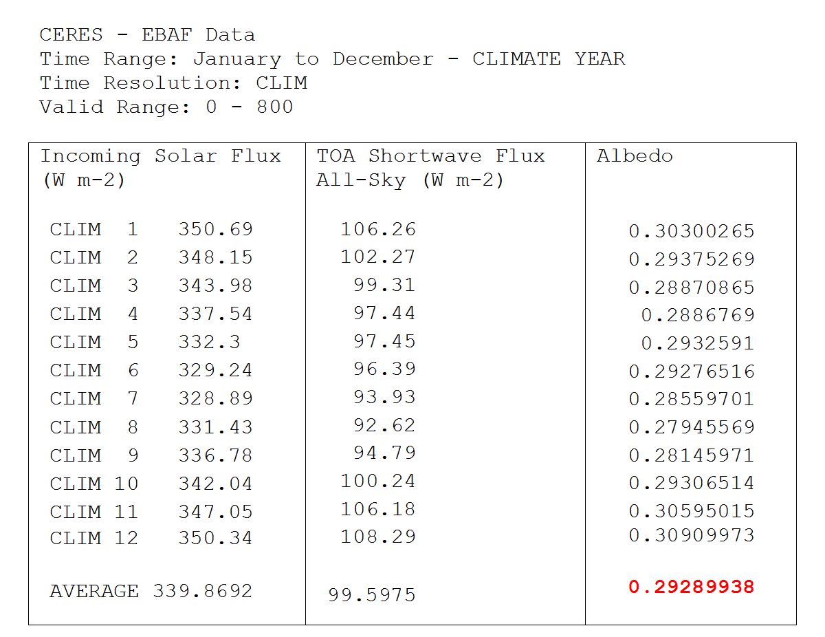
4.
A symmetrical and constrained planetary albedo at
albedo = 1 - sin 45° = 1 - √2/2 = 0.292893
Theoretical and observed values are statistically indistinguishable:
***
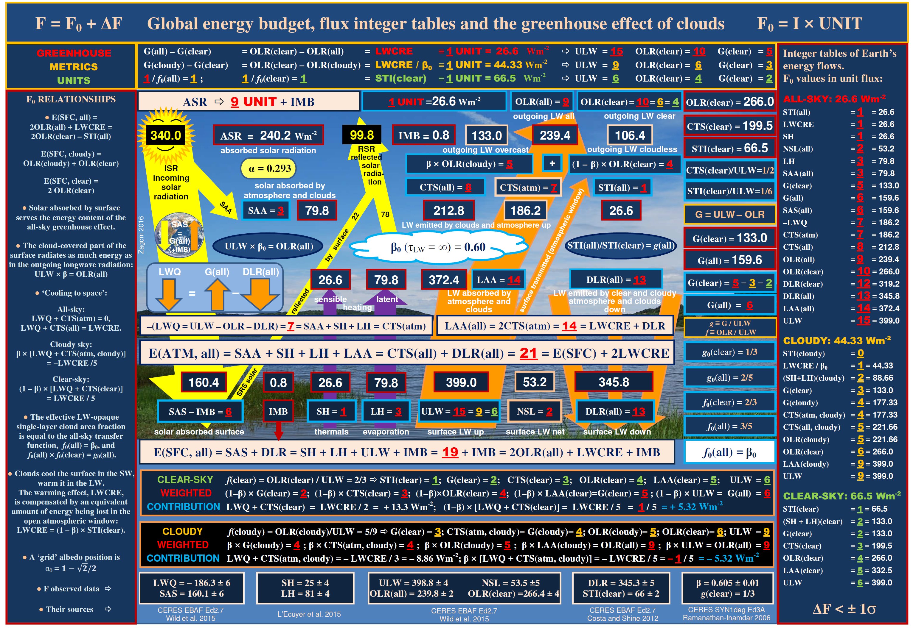
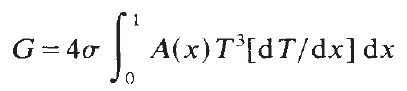
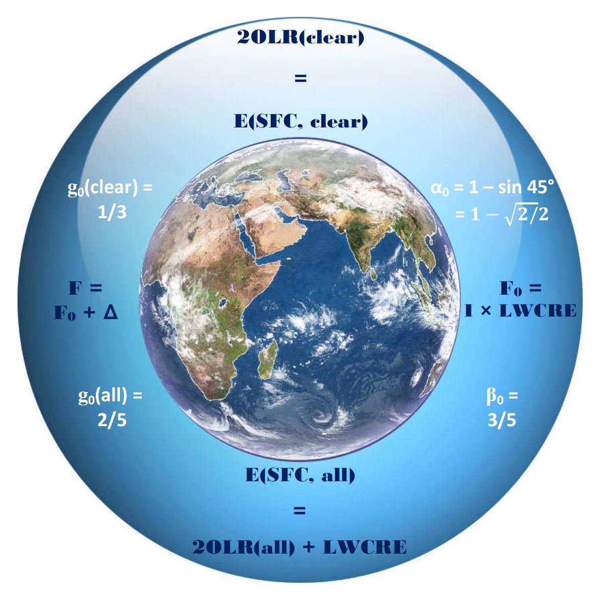
4. COMPLETE SOLUTION:
New Global Energy Budget Poster
Zagoni 2016:
(click to enlarge):
***
5. DISCUSSION, FURTHER DIAGRAMS
| OBSERVED | THEORETICAL 1 = UNIT = 26.6 W/m2 |
ULW = 2ATM(clear), SFC Net (clear) = 2WIN(clear)
*
Integer flux structure and all-sky surface energy budget in
Stephens and L'Ecuyer (2015)
(our additions in text boxes)
The following slides are from:
Martin Wild, CERES Science Team Meeting, ECMWF
(Earth Radiation Budget Workshop, UK, October 21, 2016)
our additions below in green
|
CLEAR SKY:
solar absorbed surface + thermal down surface + imbalance = 2 × thermal outgoing TOA
216 + 314 + 1 = 531 = 2 × 266 (-1) (W/m2)
G = ULW - OLR = 132 = surface net (sensible + latent)
*
*
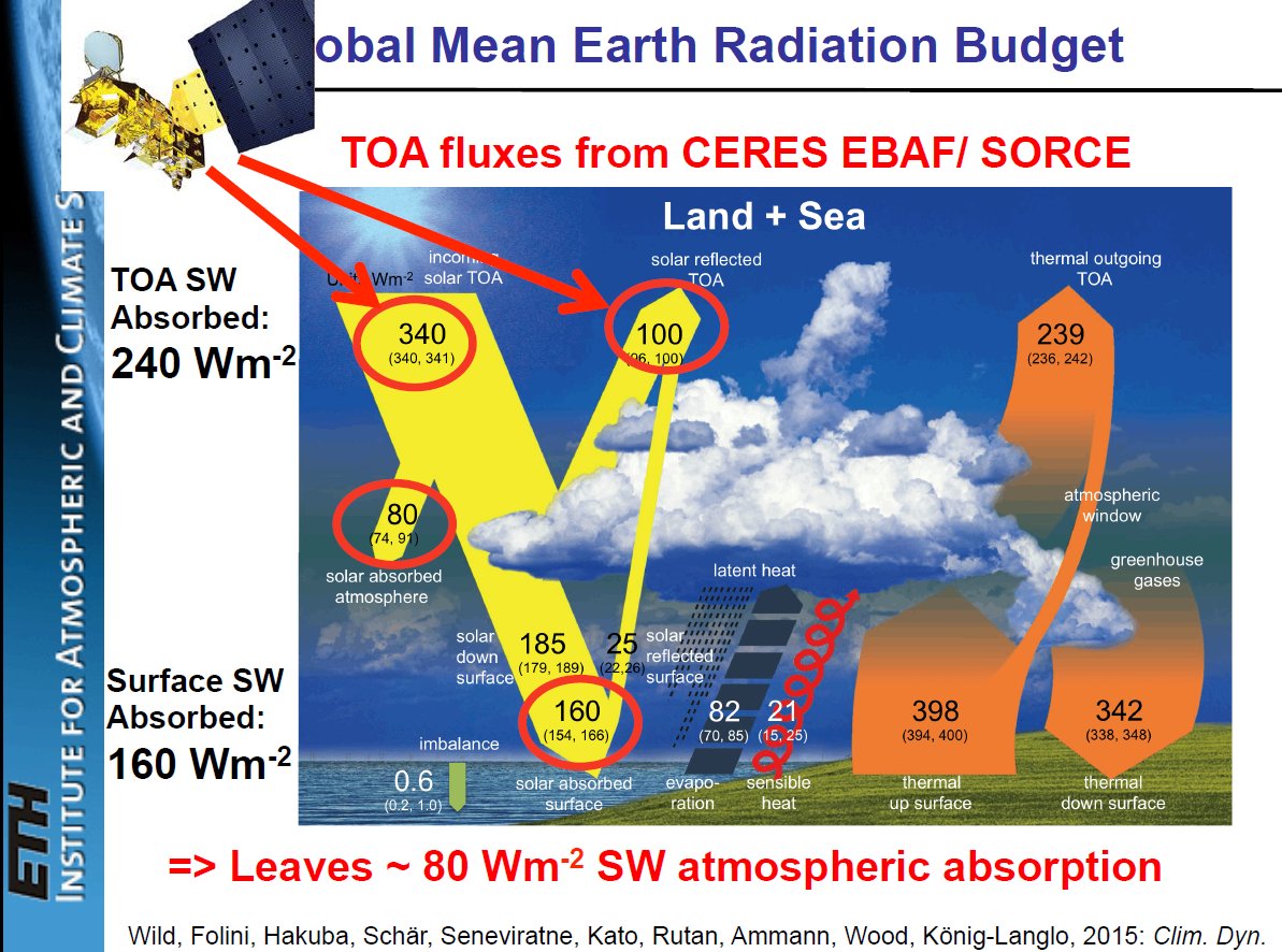
| solar absorbed atmosphere (SAA(all)) | 79.8 W/m2 | 3 UNITS |
| surface net radiation (SH + LH)(all) | 106.4 W/m2 | 4 UNITS |
| solar absorbed surface (SAS(all)) | 159.6 W/m2 | 6 UNITS |
| thermal outgoing TOA (OLR(all)) | 239.4 W/m2 | 9 UNITS |
| thermal outgoing TOA (OLR(clear)) | 266.0 W/m2 | 10 UNITS |
| thermal down surface (DLR(all)) | 345.8 W/m2 | 13 UNITS |
| thermal up surface (ULW) | 399.0 W/m2 | 15 UNITS |
| greenhouse effect (G(clear)) | 133.0 W/m2 | 5 UNITS |
| greenhouse effect (G(all)) | 159.6 W/m2 | 6 UNITS |
| TOA LW CRE | 26.6 W/m2 | 1 UNIT |
*
*
*
SW abs + LW down = 160 + 342 = 502 = Turbulent + Thermal up = 103 + 398 ( + imb)
6 + 13 (UNITS) = 4 + 15 (UNITS) = 6 + (4 + 9) = 4 + (6 + 9) = 19 UNITS
= 2 × 9 UNITS + 1 UNIT = 2OLR(all) + LW CRE = 2OLR(clear) - LW CRE
1 UNIT = ASR/9 - IMB = 26.6 W/m2
Closed glass shell geometry, modulated by LW CRE
**
*
161 decreases to 6 quanta = 159.6 W/m2
342 increases to 13 quanta = 345.8 W/m2
1 quantum = OLR/9 = 26.6 W/m2
And one from the latest, Wild (2017)
(our additions in textboxes):
Surface energy budget, E(SFC, all) =
SW↓ + LW↓ = nonrad↑ + LW↑ = 2OLR + LWCRE
6 + (4 + 9) = 4 + (6 + 9) = 2 × 9 + 1
Fluctuates around the equilibrium
*
Theory ("The Physical Science Basis")
It is unequivocal that the surface radiation budget of our quasi-aquaplanet is connected to the top-of-the-atmosphere fluxes. This connection is evident both in the clear-sky part of the atmosphere and in the all-sky mean. The TOA fluxes are known from satellite observations, the surface fluxes are determined from various independent sources. The Earth's atmosphere follows the simplest 'closed glass shell' model, and this geometry predetermines the fluxes of the global energy budget. No direct influence from changing atmospheric greenhouse gas composition can be observed.
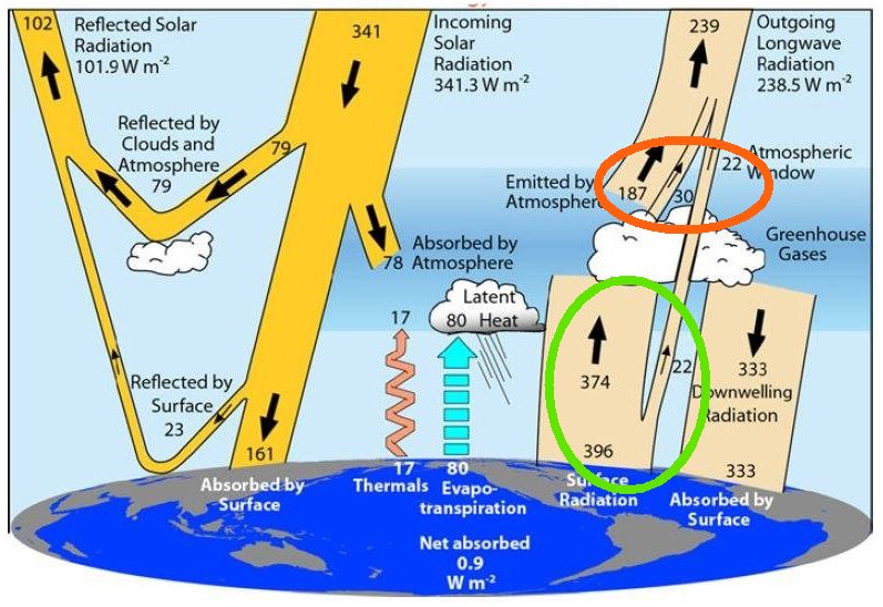
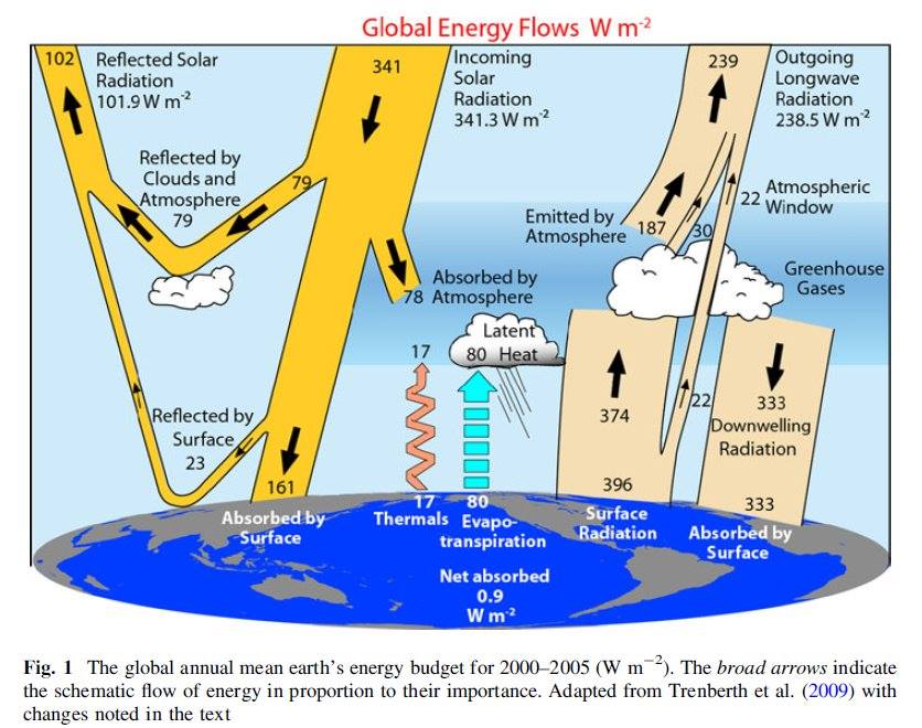
(source: Trenberth and Fasullo 2012)
In the Earth's atmosphere 374 out of 396 surface radiation is absorbed, showing a 94% IR-opacity.
The LW-effect of clouds closes the atmospheric window, making the atmosphere effectively opaque.
According to the energy minimum principle, the hot surface of Earth in a colder environment must cool as efficiently as it can. The most efficient way of cooling is direct energy transport to the coldest part of the environment (where the largest temperature difference exists): to space. Therefore the system tries to maximize surface transmitted irradiance. This requires the widest atmospheric window, that is, the driest, cloudless air. On the other hand, the surface also tries to maximize its latent cooling (evaporation), leading to the most water vapor in the atmosphere (wettest air). As long as there are sufficient water vapor supply at the surface, these two contradicting processes will balance each other at an equilibrium, prescribed by the boundary conditions. This boundary condition is the effective energetic IR-opaque limit (glass shell geometry). In one hand, the 'hole' in the atmosphere for surface direct cooling is kept (by the open IR atmospheric window); on the other hand, this window is closed by the help of a partial cloud cover, up to the 100% IR absorption.
It is remarkable that our quasi-aquaplanet is able to reproduce
the closed-shell model even in the leaky, cloudless part of the
atmosphere, and, including the greenhouse effect of a partial cloud
cover,
it exceeds the E(SFC) = 2ASR model with one LWCRE in the all-sky mean.

From this point of view, the accepted theory seems to be wrong
as presented, for example, in these two diagrams
(UK Royal Society and US Global Change reports):
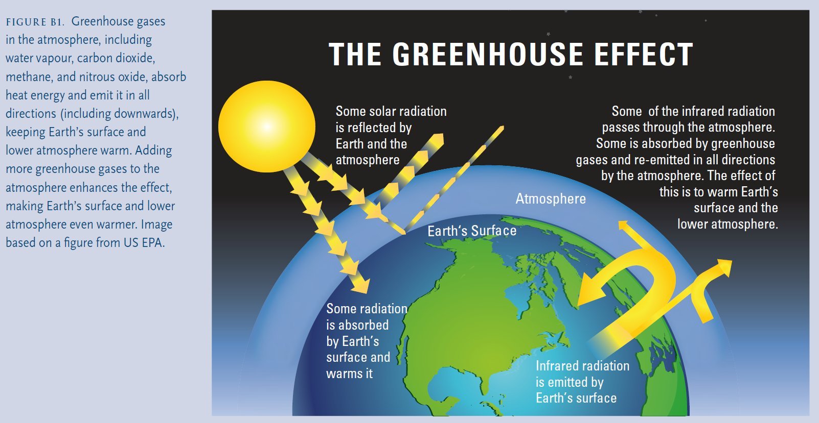
Source: Figure B1 from Climate Change: Evidence & Causes, 2014. Basics of climate change.
An overview from the UK Royal Society and the US National Academy of Sciences.
No atmospheric solar absorption, no sensible and latent heat, no clouds and — no data !
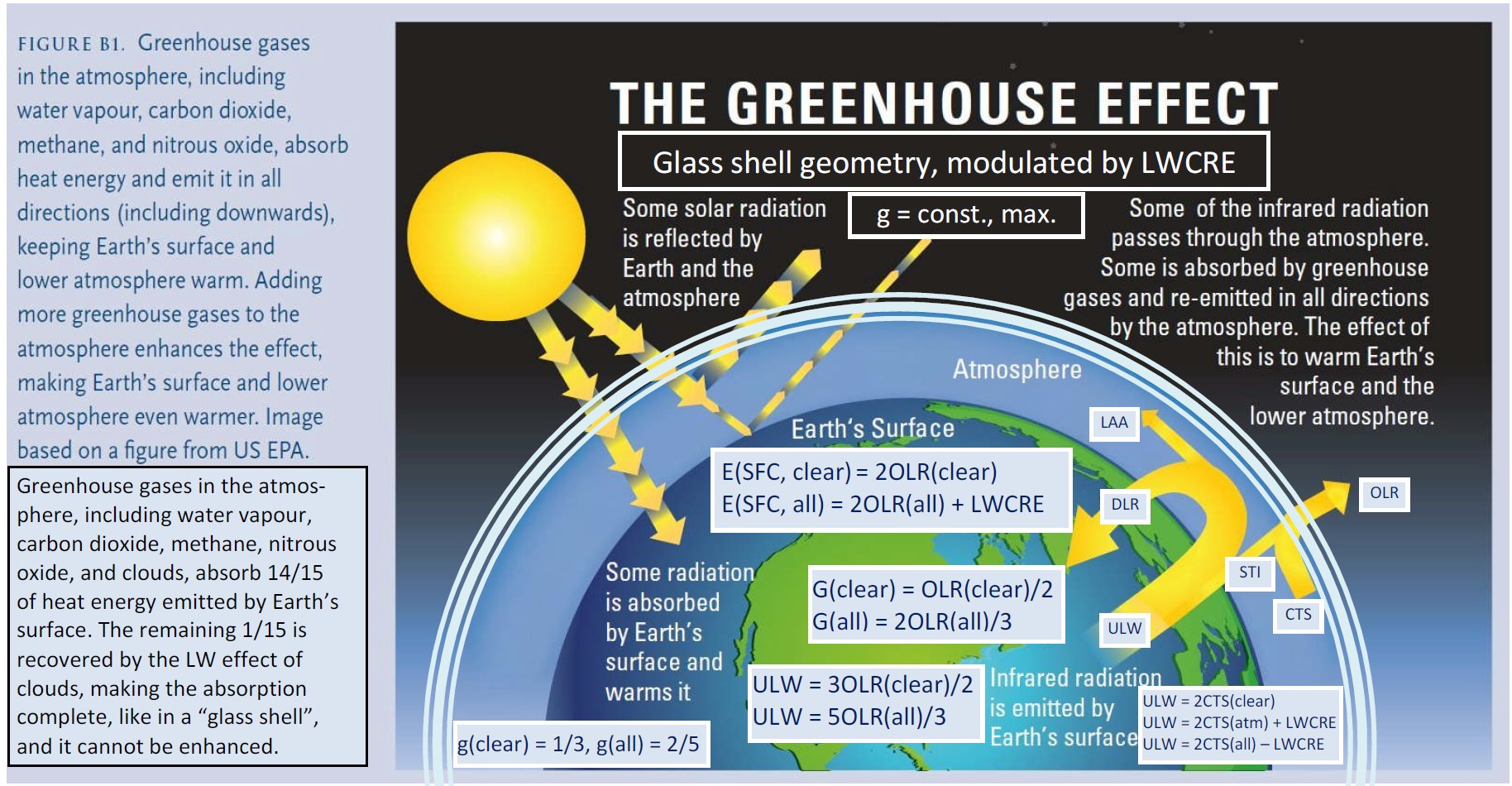
In reality, with the help of the maximized latent heat release and a partial cloud cover,
the Earth's atmosphere adjusts itself to the upper infrared absorption limit,
as if it were closed into an SW-transparent, LW-opaque glass shell
(our additions in boxes):
***
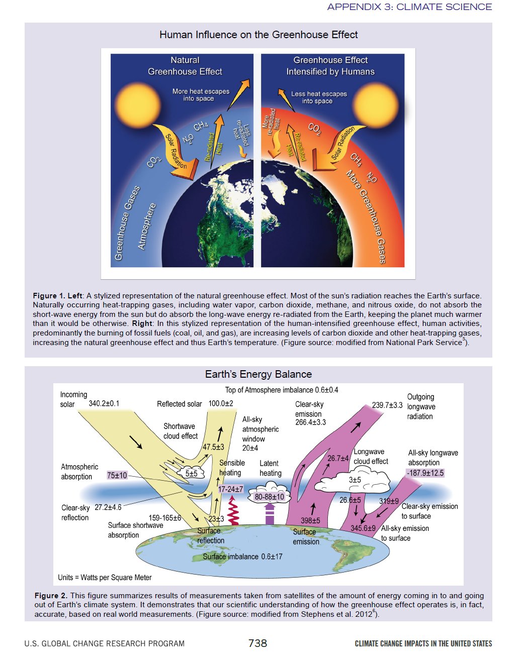
U.S. Global Change Research Program 2014,
similar problems: no H2O, no turbulent heat flows, no clouds.
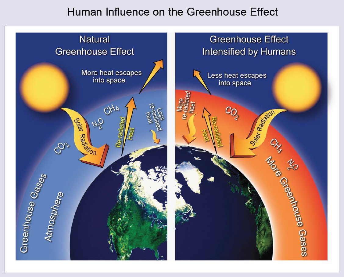
Climate Change Impacts in the United Sates,
Appendix 3: Climate Science Supplement
(Our additions in boxes):
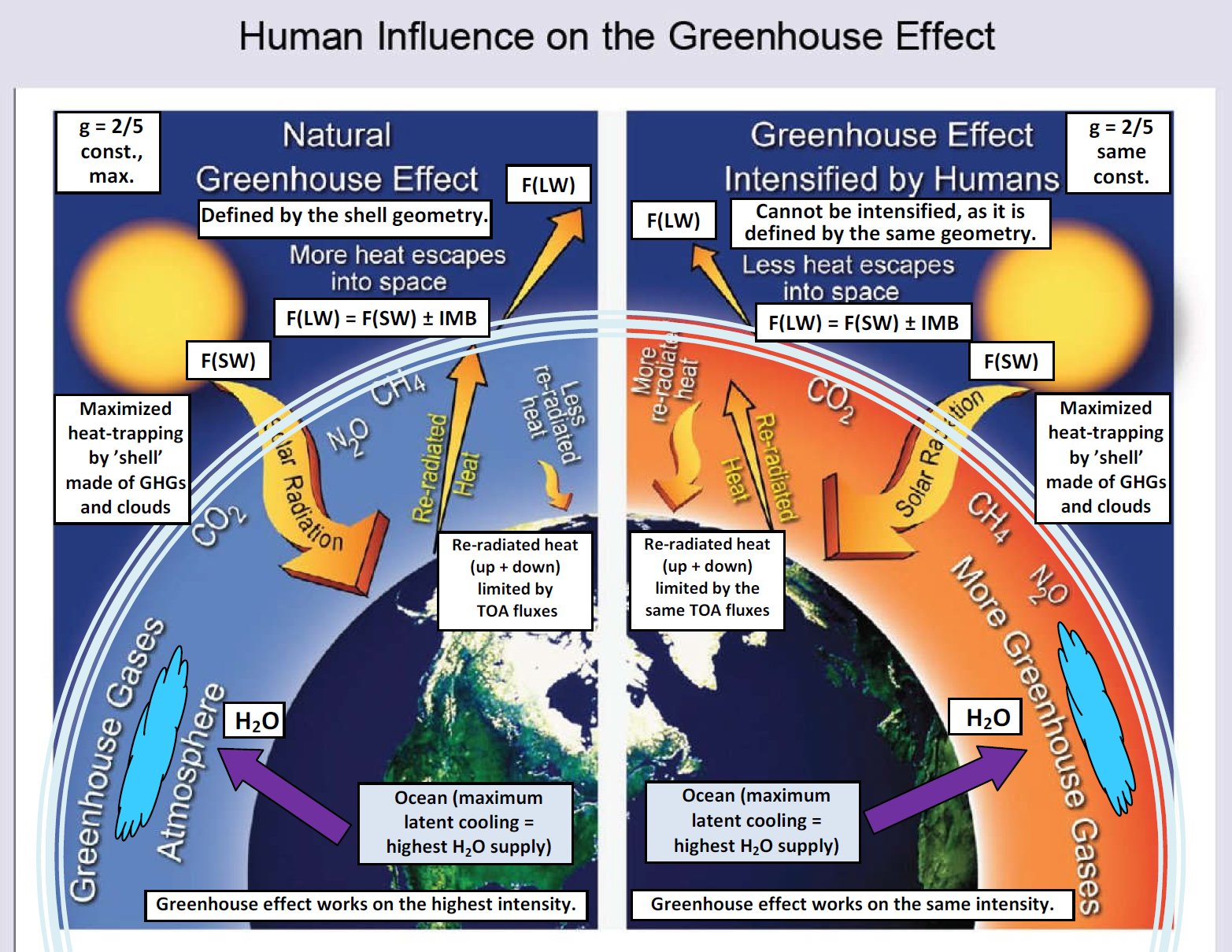
According to CERES data:
the natural greenhouse effect works on its highest possible intensity, defined by the 'glass shell' geometry,
and it cannot be intensified further. Only temporal fluctuations (imbalances) are possible.
Earth's energy budget works in a steady state.
*
The figure above in the report appeared on the same page as the Stephens et al. (2012) diagram:
But, as we have already seen, this relationship:
shows that the total atmospheric
absorption (and hence, 're-radiation', emission)
is prescribed by the upper boundary conditions: it is constrained to the TOA fluxes.
If this is so, human intensification of the greenhouse effect is not possible.
More 'heat-trapping' gas within the atmosphere cannot make it more opaque than 100%.
One can increase the left-hand side of the equation only by increasing the right-hand side.
No greenhouse effect enhancement is possible without increased absorbed solar radiation.
***
In the simplest glass shell model, the surface and TOA fluxes are connected as:
E(SFC) = 2OLR.
In the realistic, partially cloud-covered Earth case,
according to the CERES data
the greenhouse factor is predetermined by this geometry:
E(SFC, clear) = 2OLR(clear);
E(SFC, cloudy) = OLR(clear) + OLR(cloudy);
E(SFC, all) = OLR(clear) + OLR(all).
***
In the simplest glass shell model (no turbulent fluxes),
the surface energy budget is equal to the surface LW emission:
E(SFC) = ULW
and is equal to two OLR:
ULW = 2OLR,
where OLR is equal to the F solar flux,
OLR = F.
Their difference (the greenhouse effect) equals to the solar flux absorbed by the surface:
G = ULW – OLR = F.
This feature is also kept by the Earth's geometry:
the all-sky greenhouse effect equals to the solar flux absorbed by the surface:
G(all) = SAS(all).
***
The regulation starts on the solar radiation level,
and continues in its transformation into longwave and turbulent fluxes:
- shortwave reflection in the clear and the cloudy atmospheric and surface regions are controlled,
with a result of constrained global planetary albedo;
- absorption in the clear and cloudy regions, together, with the given cloud area fraction,
results in a 3/6/9 ratio for the all-sky atmospheric / surface / total solar absorption;
- surface absorption in the clear-sky region results in 8/12/20 ratio for the
shortwave / longwave / total surface absorption;
- surface emission in the clear-sky region results in a 5/15/20 ratio for the
turbulent / longwave / total surface emission;
- surface emission in the all-sky mean results in a 4/15/19 ratio for the
turbulent / longwave / total surface emission;
- TOA outgoing LW radiation in the clear-sky region shows a 1/2/3/4 ratio for
surface transmitted (window) / turbulent / atmospheric upward emission / OLR;
- all-sky Bowen ratio = SH/LH = 1/3;
- surface SW absorption in the all-sky mean equals to the LW greenhouse effect;
- surface turbulent emission in the clear-sky part equals to the clear-sky greenhouse effect.
An
intricate cooperation of the shortwave and longwave cloud properties,
together with the regulation of latent heat release, atmospheric
water vapor content and lapse rate
results in an effectively closed
shield geometry.
This is the model we can see in the constrained energy budget relationships, in the LWCRE-modulated integer flux structure, in the constrained clear-sky and all-sky infrared transparency and planetary emissivity, the regulated cloud area fraction and in the prescribed albedo, determined by the geometry.
***
Therefore, we must think that the projected increase cannot happen:
***
Our atmosphere works as an entirely IR-opaque closed 'glass' shell,
made from water vapor, GHGs and clouds.
The greenhouse effect – thermal absorption by the greenhouse gases alone – is not saturated.
Augmented by the longwave cloud effect, it is.
The greenhouse effect of gases plus the greenhouse effect of clouds, together,
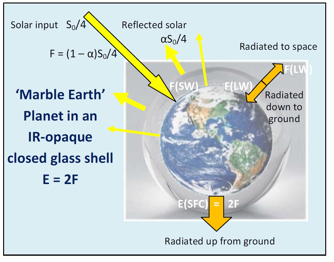
make the thermal absorption maximized and complete.
The work of the
'Marble Earth'
E(SFC) = 2OLR
geometry
in reality (leaky, turbulent) in the clear-sky part:
E(SFC) = ULW + Turb = 2 OLR = 2 ATM + 2 WIN
ULW = 2 ATM, Turb = 2 WIN.
Clouds in reality are almost IR-opaque objects (depending on their composition and thickness):
their presence in a certain amount is able to make the 'leaky' atmospheric regions non-transparent.
But their LW-effect is twofold: they radiate downward as well as upward.
Therefore the 'substitution' of the window radiation with cloud-radiation adds an extra,
but prescribed amount of LW energy to the system:
E(SFC, all) = 2OLR(all) + LWCRE.
As a result, the whole energy flow structure is predetermined by the
boundary conditions, where all the internal fluxes: shortwave and longwave, radiative and turbulent,
including the greenhosue effect for the clear-sky and the cloudy parts of the atmosphere,
show a certain periodicity, modulated by a given unit flux or 'quantum'.
The greenhouse surplus at the surface is G↑ = ULW - OLR = 15 - 9 = 6 units,
being equal to G↓ = DLR + LWQ =
the sum of LW Heating (13) and LW Cooling (-7) = G = 13 - 7 = 6 units,
and equals to solar absorbed surface, SAS = ASR - SAA = 9 - 3 = 6 units.
The IR-opaque partial cloud layer increases the glass-shell (E = 2OLR) energy budget with
the longwave effect of clouds:
The surface energy budget is
E(SFC, all) = 2OLR(all) + LWCRE;
The atmospheric energy budget is
E(ATM, all) = CTS(all) + DLR(all) = 2OLR(clear) + LWCRE.
***
'Cloud' in theory is a single, completely IR-opaque partial layer;
the values above are idealized ratios related to that geometry with a 2/5 clear-sky fraction;
OLR(all) = 239.4 W/m2.
'Cloud' in observation may include thin objects with low visible optical depth and non-zero IR transparency.
Cloud fraction = 0.67, if the visible optical depth > 0.1,
Increases to 0.74 if objects included with SW optical depth < 0.01,
decreases to 0.56 for clouds with visible optical depth > 2.
Cloud fraction is about 0.6 for τSW > 1 and τLW >> 1.
From an energetic point of view, STI(all) is lost through the atmospheric window, LW CRE tries to make the patchwork.
If “climate is what you expect, weather is what you get”, then
STI(all) is what you expect, LW CRE is what you get.
Their local, temporal, regional and annual differences in the dynamics of the climatic energy flow system
influence the global energy balance, but the basic determinations are given by the boundary conditions.
Vibrations around the crystal-lattice positions are possible in unknown size and time-scale.
Our personal comments
(Original: M. Wild, CERES Science Team Meeting, Oct 2016. Our additions in red).
With respect, it is hard to believe that Dr Wild did not realize this relationship,
or that he wouldn't know what does it mean. But on what physical basis?
We were not able to find any reference to this identity in the literature.
*
Dr Loeb's diagram (2014):
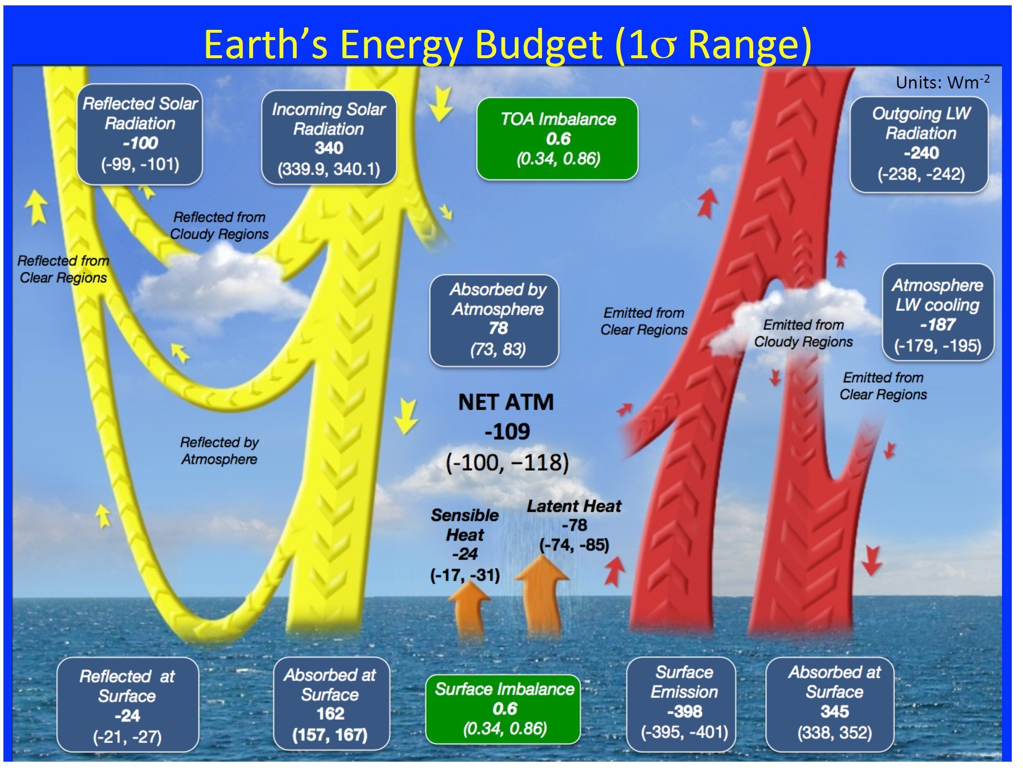
ASR = 240 ± 1, SAA = 78 ± 5, SAS = 162 ± 5, SH = 24 ± 7, LH = 78 ± 6, ULW = 398 ± 3,
DLR = 345 ± 7, LW cooling = 187 ± 8, NET ATM = 109 ± 9 , (SH + LH = 102 ± 7), OLR
= 240 ± 2
E(SFC) = 162 + 345 = 398 + 109 = 507 = 2
× 240 + 27 = 2OLR + LWCRE,
very close fit.
Theoretical (quantized) values (with ASR = 240.0 and IMB = -0.6):
SH = 26.6, LH = 79.8; SH + LH = 106.4, SAA = 79.8, SAS = 159.6, LW
cooling = 186.2
OLR = 239.4, DLR = 345.8, ULW = 399.0
*
These are surface - TOA correlations.
The atmosphere - TOA version of these identities, as mentioned earlier,
can be found in the Stephens et al. (2012) diagram
(co-authors M Wild, N Loeb, S Kato, T L'Ecuyer et al.):
and this NASA LaRC diagram (2014):
Our additions:

Again, it is hard to imagine that this relationship is not a result of intentional adjustment,
or that the authors (the NASA LaRC science team, 2014) were not aware of what does it mean.
*

And again: it is hard to believe that this relationship is not a result of intentional adjustment,
or that the authors (N. Loeb, S. Kato et al.) were not aware of what does it mean.
*
It is hard to believe that this relationship is not a result of intentional adjustment,
or that the authors (N. Loeb, S. Kato et al.) were not aware of what does it mean.
*
It is hard to imagine that this match is not deliberately adjusted.
The expression of f(clear) = 2/3 is equivalent to g(clear) = 1/3, or 2G(clear) = OLR(clear).
This relationship expresses very plainly that G(clear) is predetermined by OLR(clear).
We must think that the authors (N. Loeb, S. Kato et al.) were aware of this fact.
*
If the sum of atmospheric up and down emissions, or the surface absorptions, or the greenhouse effect, is constrained to OLR,
then no internal increase of these energy flows is possible.
Therefore, any of these equalities would destroy the accepted theory about the enhanced greenhouse effect.
***
TERMINOLOGY
So far we handled the different graphical representations
(global energy budget diagrams) as basically equivalent.
But they are not; there are essential conceptual differences.
 Trenberth and Fasullo (2012). Emitted by Atmosphere (upward): 187, LW Absorbed by Atmosophere: 374. | 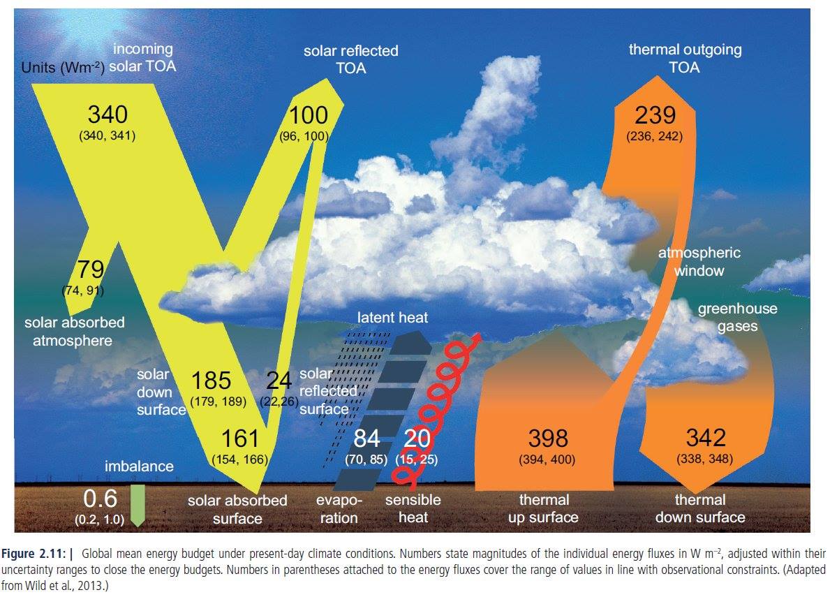 Wild et al. 2013 (IPCC 2013) Neither Emitted by Atmosphere (upward), nor LW Absorbed by Atmosphere is given. |
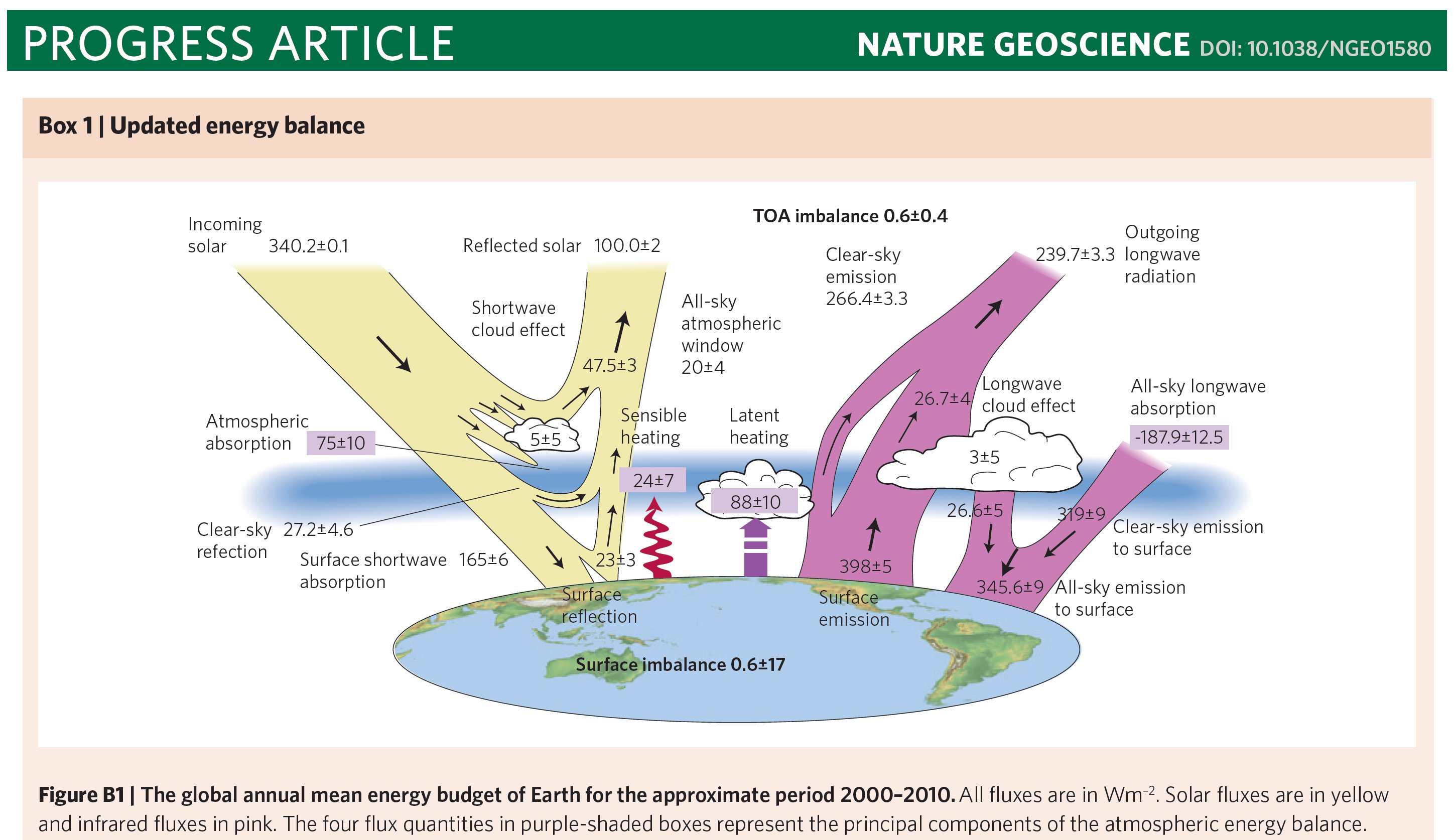 Stephens et al. (2012). No Emitted by Atmosphere (upward) is shown, the flux called 'All-sky longwave absorption' = -187.9, is defined as LW Cooling = ULW - DLR - OLR; the negative sign indicates that it is an (upward) emission. | Stephens and L'Ecuyer (2015) Neither Emitted by Atmosphere (upward), nor LW Absorbed by Atmosphere is given, LW Cooling is presented as -185. |
 NASA LaRC (2014) Like Trenberth and Fasullo 2012, but with wrong 'atmospheric window'. | 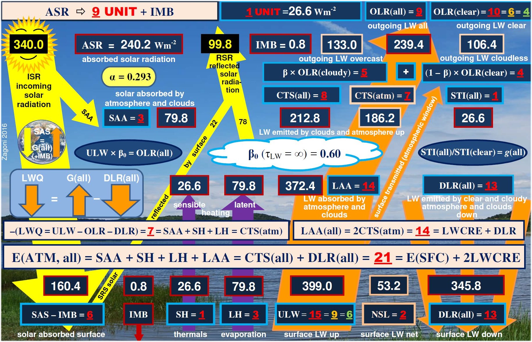 Our diagram (Zagoni 2016) We hoped to solve the above inconsistencies within a coherent terminology. |
The observable flux elements in the budget are well-understood, and there is consensus in their representation.
But there are differences in the only-computable fluxes such as upward atmospheric emission. In the Trenberth (2012) diagram its value is 187 W/m2, but there is neither label nor number for this flux in the IPCC 2013 (Wild et al.) diagram; at least a vector is representing this energy flow. In the Stephens et al. (2012) figure even this flow is missing: OLR doesn't add up, it has a window and an LWCE component, but that's all. One may guess whether the negative value for the 'All-sky longwave absorption' (-187.9) might mean actually an emission (with a value of +187.9)? According to its numerical value, it is LW cooling in the Stephens and L'Ecuyer (2015) diagram (= ULW - DLR - OLR), being equal further to the atmospheric solar + turbulent heat uptake. We examine this question in more detail at the main site in the Cooling-To-Space section (as also described in our poster).
***
FURTHER PROBLEMS
can be found in the determinations of
the greenhouse effect and DLR in a CERES documentation:
Algorithm Theoretical Basis Document
Estimation of Longwave Surface Radiation Budget From CERES
(Subsystem 4.6.2)
CERES Science Team Surface Radiation Budget Working Group
Principal Investigators
A. K. Inamdar
V. Ramanathan
June 2, 1997
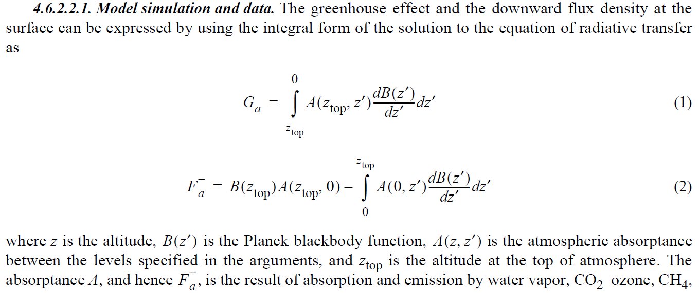
The list of symbols correctly defines the greenhouse effect
and the downward LW flux density as:
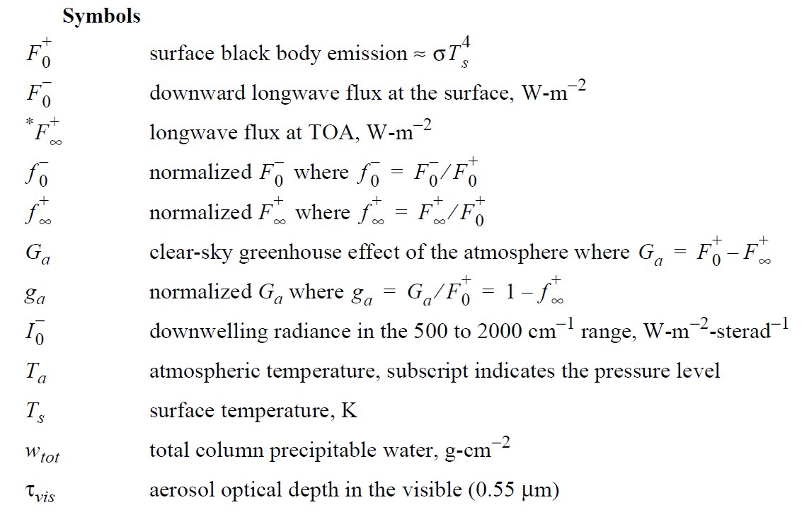
but the given equations (1) and (2) define another quantities:
The source of the problem can be traced back to a NATURE-paper (cited by the document):
Raval and Ramanathan (1989):
Observational determination of the greenhouse effect.
This paper introduces the concept of 'heat trapping':
"Satellite measurements are used to quantify the atmospheric greenhouse effect,
defined here as infrared radiation energy trapped by atmospheric gases and clouds."
First, G is correctly defined as G = B(Ts) - F, that is,
G = ULW - OLR, where the TOA flux (OLR) is given as:
and B(Ts) is the LW flux emitted by the surface (ULW).
Here A(x) is the absorptivity between TOA and level x. Hence
But this formula desribes LW atmospheric absorption (LAA), instead of G,
leading to a long queue of misunderstandings and misinterpretations.
*
SUMMARY
“The greenhouse effect is best illustrated from the annual and global average radiative energy budget. At a global average surface temperature of about 289 K, the globally averaged longwave emission by the surface is about 395 +/-5 Wm-2, whereas the OLR is only 237 +/- 3 Wm-2. Thus, the intervening atmosphere and clouds cause a reduction 158 +/-7 Wm-2 in the longwave emission to space, which is the magnitude of the total greenhouse effect (denoted by G) in energy units.” (Volvo Prize Lecture, 1997)
Note
that g = G/ULW = 158/395 = 0.4. This value is exactly the same
as today and equals to the theoretical value of 2/5 (6/15 units, see our tables and diagrams above). No increase in strength of
the greenhouse effect during these two decades.
Add more CO2 into the atmosphere; what's happening? More IR-absorption -> immediate (instantaneous? seasonal? annual?) radiative response from the boundary constraints -> internal reorganisation (water cycle?) -> annual mean integer flux structure maintained -> stability restored. It seems that the surface temprerature rise is missing from the feedback loop.
Further research is needed to determine that (a) under the same annual global mean, what kind of seasonal, vertical and regional changes in water vapor, temperature and cloudiness distributions might be caused by the increasing CO2-amount, (b) how long and large deviations (fluctations) are possible around the steady-state (F0) positions described above (predetermined by the geometry), and (c) what factors might lead to profound reorganisations like glacial and interglacial transitions.
Miklos Zagoni
email: info@globalenergybudget.com
Note that the distance of the "shell" (the origin of OLR) from the Earth's surface in reality is about 5.5 km; the area correction factor is (6371/6371+5.5)2 = 0.9983. That is, 239.6 W/m2 at the surface is 239.2 W/m2 at the level of the origin of outgoing longwave radiation. The difference is 0.4 W/m2.
*
* *
* * *
Have some fun:
Climate Quarks
* * *
* *
*
Continue reading on the main site: Foreword, Abstract, Introduction.