Validation

Validation of Eq. (1) and Eq. (2) on model RE and real RCE conditions

“The Eddington approximation will generally be employed; while it is not precise it omits no
essential physical principles, provided that the medium is stratified.” — Goody (1964)

Equation (1)

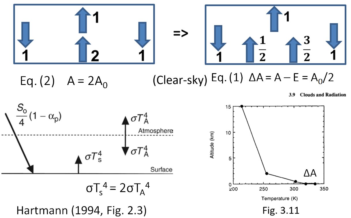
Dennis Hartmann in his book Global Physical Climatology (1st ed. 1994, 2nd ed. 2016) gives a stratified two-layer radiative equilibrium model:

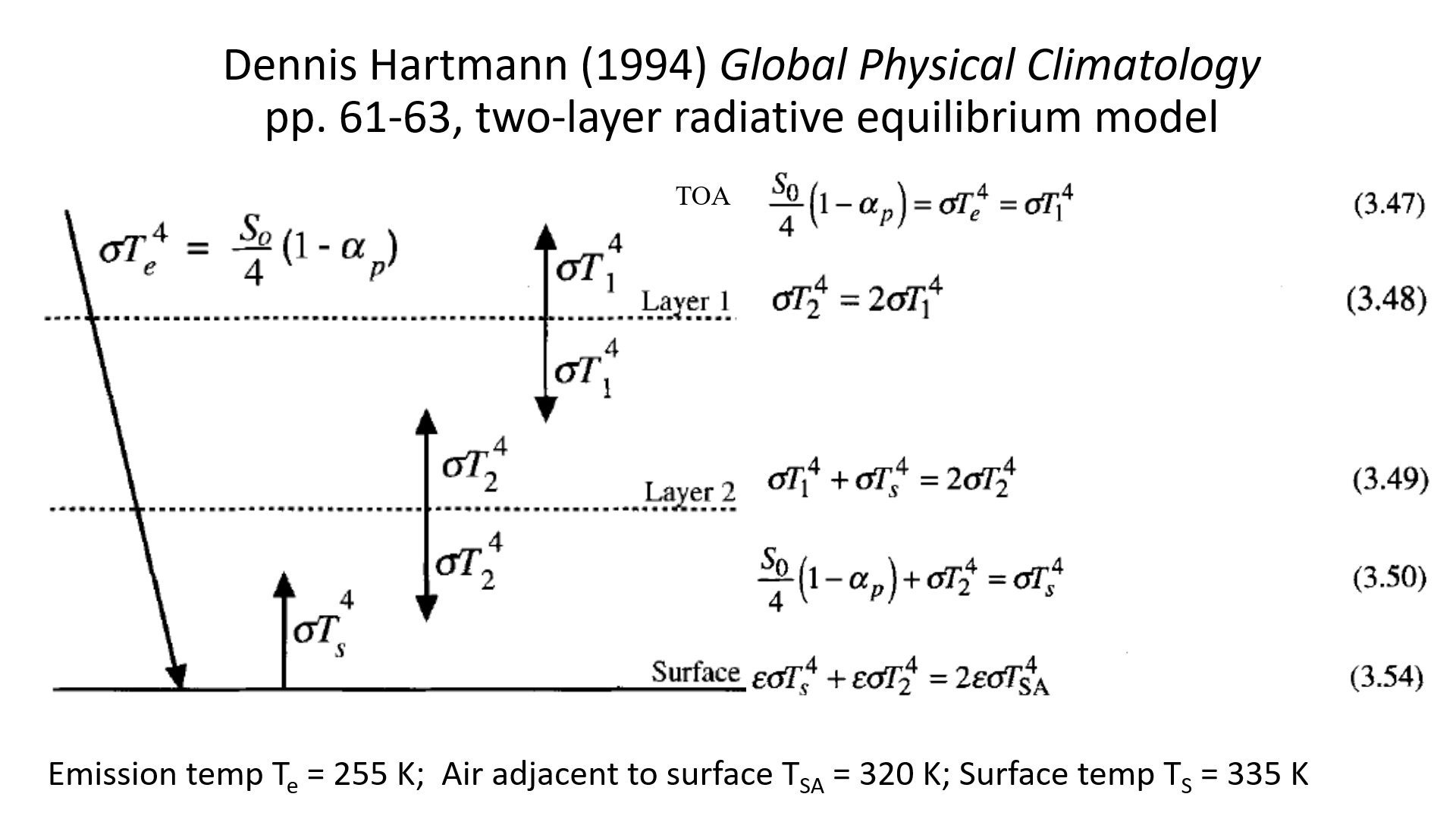
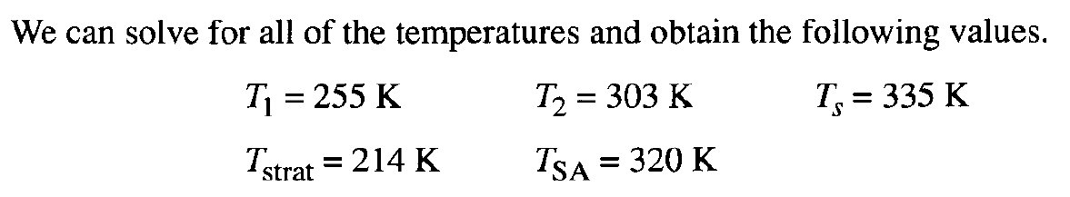
Assuming an emission temperature Te = 255 K as input parameter, the resulted temperatures are calculated according to the given equations.

The temperature of the air layer adjacent to the surface is Tsa = 320 K, and the surface temperature is Ts = 335 K.

For all the given temperatures,

σT_strat⁴ = 118.92 Wm-2; σT₁⁴ = σT_e⁴ = 239.74 Wm-2; σT₂⁴ = 477.92 Wm-2; σT_SA⁴ = 594.54 Wm-2; σT_s⁴ = 714.11 Wm-2; hence

T_strat⁴ : T₁⁴ : T₂⁴ : T_SA⁴ : T_s⁴ = 1 : 2 : 4 : 5 : 6.

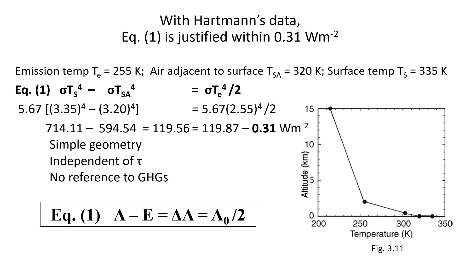
With these approximative data, Eq. (1) is satisfied by a difference of 0.31 Wm-2.

σT_s⁴ – σT_SA⁴ = σT_e⁴ /2

5.67 × [3.35)⁴ –(3.20)⁴] = 5.67 × (2.55)⁴ /2

714.11 – 594.54 = 119.56 = 119.87 – 0.31 Wm^-2.

Hartmann (1977, Fig. 3.11) shows ΔA (the flux discontinuiiy, temperature jump) at the surface in radiative equilibriium:

Eq. (1) and eq. (2): Validation on CERES EBAF Data in Earth's Radiative-Convective Equilibrium conditions:

When we first encountered this problem, CERES EBAF Edition 2.8 data set was available.
We took the clear-sky data from a CERES science team meeting presentation of Rose et al. (2017).

In this notation,

Eq. (1) SFC SW Down – SFC SW Up + SFC LW Down – SFC LW Up = TOA LW Up /2

Eq. (2) SFC SW Down – SFC SW Up + SFC LW Down = 2 x TOA LW Up.

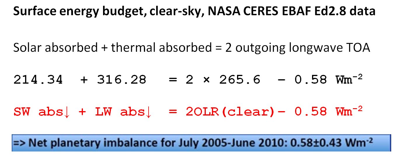
Clear-sky, Ed2.8 data (here we show our recognition in its original form six years ago):

Eq. (1):

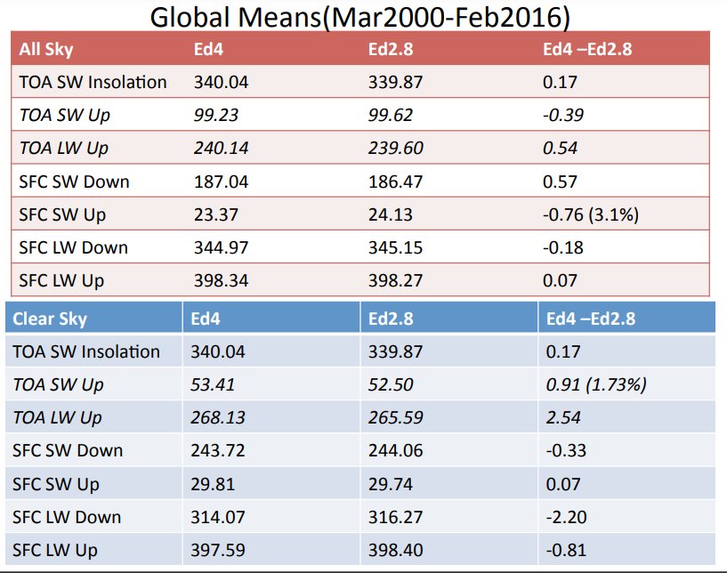
EBAF Ed4 clear-sky, from the same dataset:

Eq. (1) Surface (SW net + LW net) = TOA LW /2
243.72 – 29.81 + 314.07 – 397.59 = 268.13 /2 – 4.3 Wm-2

It seems that in this dataset, the equation is valid with the CERES instrument calibration uncertainty of 4.3 Wm-2.

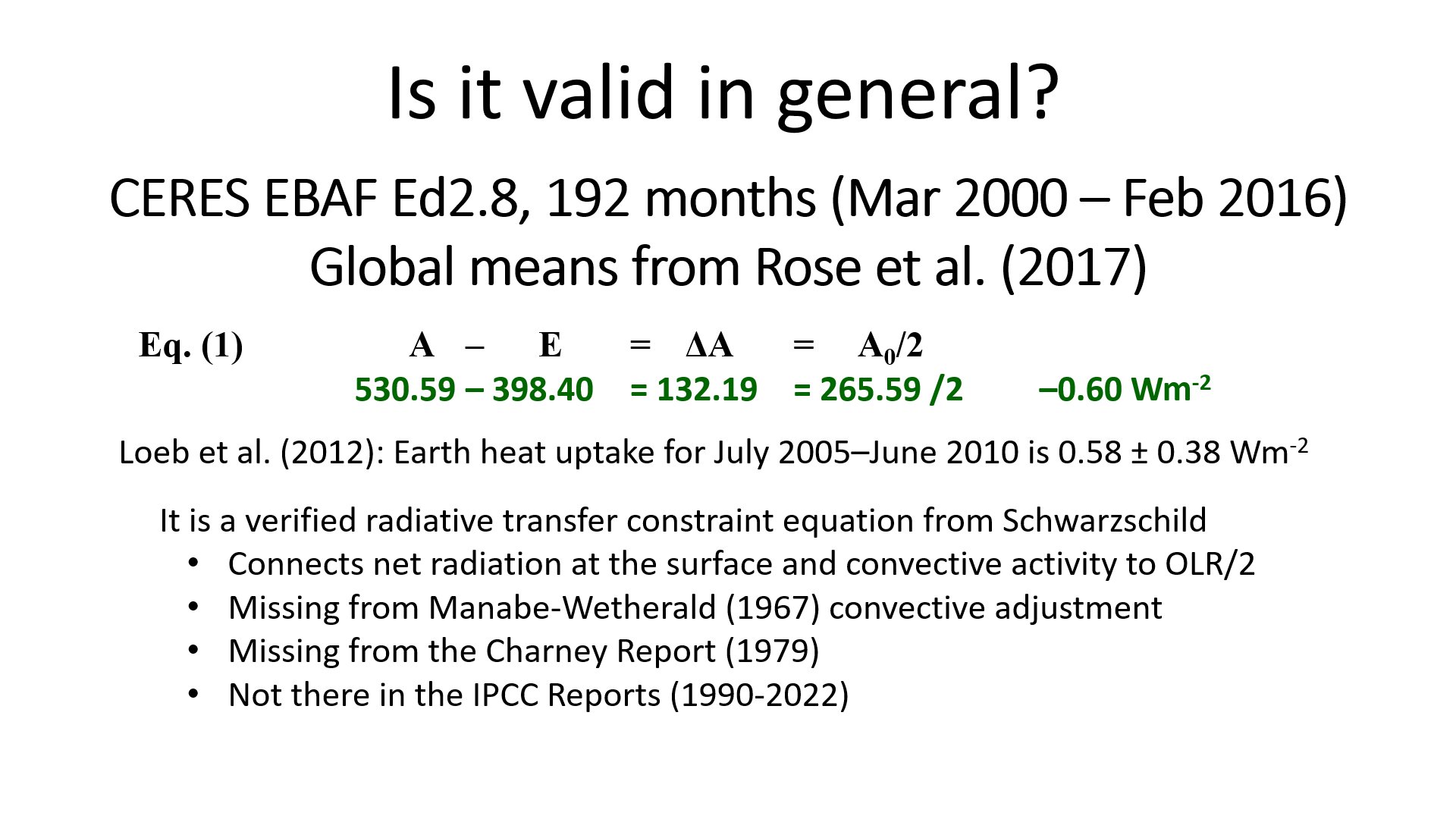
Eq. (1) is a verified radiative transfer constraint equation.

It comes directly from Schwarzschild's (1906, Eq. 11)
It connects the net radiation at the surface (and the corresponding convective activity) unequivocally to OLR/2
It does not refer to the GHGs or any atmospheric gaseous composition
It does not refer to the vertical structure of the atmosphere
It is missing from the Manabe and Wetherald (1967) convective adjustment
It is missing from all of its follow-up sensitivity studies
It is missing from the Charney Report (1979)
It is not there in any of the IPCC Reports (1990-2022).

Eq. (1) and (2):

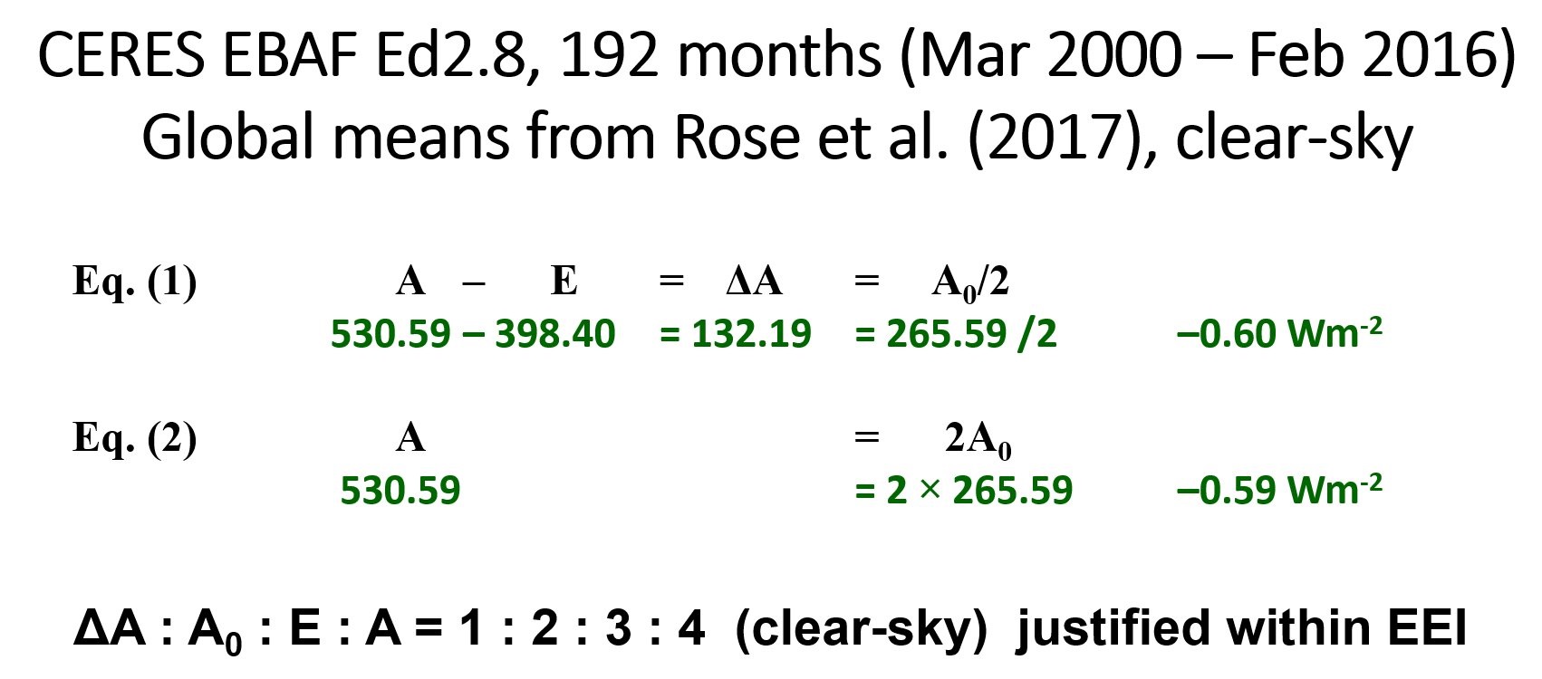
Eq. (1) 244.06 – 29.74 + 316.27 – 398.40 = 265.59 / 2 – 0.60 Wm^-2

Eq. (2) 244.06 – 29.74 + 316.27 = 2 x 265.59 – 0.59 Wm^-2.

In that time, the planetary imbalance was regarded 0.58 Wm^-2

The same accuracy of Eq. (2) as that of Eq. (1) in EBAF Ed2.8 was one of the most intriguing recognitions in our research.

In EBAF Ed4, Surface LW down was decreased by 2.20 Wm-2, while TOA LW up was increased by 2.54 Wm-2, leading to a more than 8 Wm-2 shift in Eq. (2).

Some years later, EBAF Ed4.1 balanced the deviation of the equations, as we will see soon.

Eq. (1) is "only" a known but overlooked relationship; its validity on real data is important, but in a theoretical sense, not surprising.

Eq. (2), on the other hand, expresses something really new, the validity of the optical depth = 2 case and the corresponding simplest single-layer atmospheric greenhouse geometry (see below). The geometry is defined by the GHG-independent integer ratios:

ΔA : A₀ : E : A = 1 : 2 : 3 : 4

This is the physical basis of the clear-sky ratios show in clear-sky CERES data above.

Surface net : OLR : ULW : Surface total = 5 : 10 : 15 : 20

we see in the data,
with unit flux 1 = LWCRE = 26.68 Wm-2.

Before we turn to the most recent datasets of Edition 4.1 and 4.2, let us recall the SYN1deg SFC Ed4 and EBAF TOA Ed4 data from the same time, where the original CERES instrument calibration uncertainty required a TOA flux adjustment is also indicated:

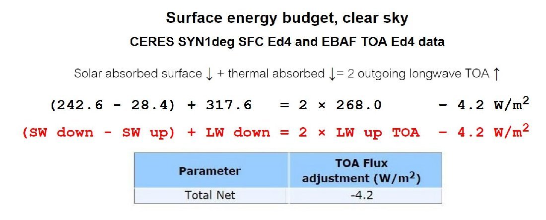
It can be concluded that Earth's global mean energy flow system satisfies these two Schwarzschild equations in the clear-sky annual global mean, according to this dataset spanning 17 years of observation, within a difference of Earth's energy imbalance.

The equations require also that E = 3A₀/2. Controlling this equation on the data:

398.40 = 3 x 265,59/2 + 0.015 Wm^-2.

We will show later in detail that here that a geometric representation of the two clear-sky equations (1) and (2) can be based on Hartmann's single-layer atmospheric greenhouse model:

The greenhouse effect is the difference of upward LW fluxes at the lower and the upper boundary (G = SFC LW Up – TOA LW Up).
According to the equations, G = E – A₀; and the normalized g = G/(SFC LW Up) = (E – A₀) / E = 1/3.
Clear-sky data: (398.40 – 265.59) / 398.40 = 0.333358.

It seems Earth's greenhouse effect is very accurately (almost precisely) equals to the theoretical one.
Notice, the theoretical model does not refer to any atmospheric gaseous composition or lapse rate.

For details, see our Spring and Fall 2020 and 2021 CERES Science Team Meeting presentations:

https://ceres.larc.nasa.gov/documents/STM/2020-04/47_Patterns4-CERES_Zagoni.pdf

https://ceres.larc.nasa.gov/documents/STM/2020-09/34_Zagoni_G5.pdf

https://ceres.larc.nasa.gov/documents/STM/2021-05/34_Zagoni_CERES_STM35.pdf

https://ceres.larc.nasa.gov/documents/STM/2021-09/26_CERES_STM_Fall21-Zagoni.pdf

On the next page, we create the all-sky versions of these two equations, and control them on the most recent CERES EABF Edition 4.1 and Edition 4.2 data products.

Go to the next page "All-sky versions " or go back to the main "index page".